Attention Is All You Need (Transformer)

Attention Is All You Need introduced the Transformer, a sequence transduction architecture built entirely out of attention mechanisms, with no recurrence and no convolution.

Paper: Vaswani, Shazeer, Parmar, Uszkoreit, Jones, Gomez, Kaiser, Polosukhin (Google Brain/Research and University of Toronto), NeurIPS 2017, arXiv:1706.03762.
Evaluation: WMT 2014 English-to-German and English-to-French machine translation.
Why it matters: the architecture nearly all subsequent large language models and vision transformers (including DETR) are built on.

Core idea

Prior state-of-the-art sequence models (RNNs, LSTMs, GRUs) factor computation along the position of the sequence: hidden state $h_{t}$ depends on $h_{t - 1}$ , which is inherently sequential and precludes parallelization within a training example. Convolutional alternatives (ByteNet, ConvS2S) parallelize but require $O (n)$ or $O (lo g_{k} n)$ layers stacked to connect distant positions.

The Transformer instead relies entirely on self-attention (also called intra-attention) to compute representations of a sequence, relating all positions to each other with a constant number of sequential operations. This buys:

Full parallelization within a training example — no step depends on the previous step’s output.
Constant path length between any two positions, versus $O (n)$ for recurrent layers, making it easier to learn long-range dependencies.
Faster training in wall-clock time despite comparable or lower total complexity, because there is nothing sequential to bottleneck it.

The tradeoff is that per-layer complexity is $O (n^{2} \cdot d)$ (quadratic in sequence length $n$ , linear in representation dimension $d$ ) versus $O (n \cdot d^{2})$ for a recurrent layer — cheaper only when $n < d$ , which is typically true for sentence-level translation.

Architecture

The Transformer follows the standard encoder-decoder structure, but both stacks are built purely from attention and position-wise feed-forward layers (see Figure 1).

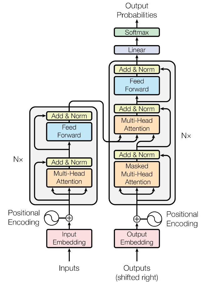
The Transformer model architecture
Figure 1 from the paper: encoder (left) and decoder (right) stacks.

Encoder: a stack of $N = 6$ identical layers. Each layer has two sub-layers: (1) multi-head self-attention, (2) a position-wise fully connected feed-forward network. A residual connection wraps each sub-layer, followed by layer normalization: the output of each sub-layer is $LayerNorm (x + Sublayer (x))$ . To make the residual connections work, every sub-layer and the embedding layers produce outputs of dimension $d_{model} = 512$ .

Decoder: also a stack of $N = 6$ identical layers, with a third sub-layer inserted per layer that performs multi-head attention over the encoder’s output (encoder-decoder attention). The decoder’s self-attention sub-layer is masked — positions are prevented from attending to subsequent positions, by setting the corresponding softmax inputs to $- \infty$ — so that, combined with the output embeddings being offset by one position, predictions for position $i$ can only depend on known outputs at positions $< i$ . This preserves the auto-regressive property at inference.

Embeddings and softmax: input and output tokens are converted to $d_{model}$ -dimensional vectors via learned embeddings. The same weight matrix is shared between the input embedding, the output embedding, and the pre-softmax linear transformation (weight tying). Embedding weights are multiplied by $d_{model}$ .

Scaled dot-product attention

An attention function maps a query and a set of key-value pairs to an output, computed as a weighted sum of the values, where each value’s weight comes from a compatibility function between the query and the corresponding key. The Transformer uses:

Attention (Q, K, V) = softmax (\frac{Q K ^{T}}{d _{k}}) V

where $Q$ , $K$ , $V$ are matrices packing together queries, keys ( $d_{k}$ -dimensional), and values ( $d_{v}$ -dimensional). This is dot-product attention identical to the standard formulation except for the $\frac{1}{d _{k}}$ scaling factor. Dot-product attention is much faster and more space-efficient than additive attention (which uses a feed-forward network with one hidden layer to compute compatibility) since it reduces to highly optimized matrix multiplication, and the two perform similarly for small $d_{k}$ . But for large $d_{k}$ , unscaled dot products grow large in magnitude — assuming components of $q$ and $k$ are independent random variables with mean 0 and variance 1, their dot product has variance $d_{k}$ — pushing the softmax into regions with extremely small gradients. Scaling by $\frac{1}{d _{k}}$ counteracts this.

Multi-head attention

Rather than performing a single attention function with $d_{model}$ -dimensional keys, values, and queries, the model linearly projects $Q$ , $K$ , $V$ $h$ times with different learned projections to $d_{k}$ , $d_{k}$ , $d_{v}$ dimensions, performs attention in parallel on each projected version, concatenates the results, and projects once more:

MultiHead (Q, K, V) = Concat (head_{1}, \dots, head_{h}) W^{O}

where head_{i} = Attention (Q W_{i}^{Q}, K W_{i}^{K}, V W_{i}^{V})

with projection matrices $W_{i}^{Q}, W_{i}^{K} \in R^{d_{model} \times d_{k}}$ , $W_{i}^{V} \in R^{d_{model} \times d_{v}}$ , and $W^{O} \in R^{h d_{v} \times d_{model}}$ . A single attention head averages over all positions, which inhibits the ability to focus on multiple different things at once; multi-head attention lets the model jointly attend to information from different representation subspaces at different positions. With $h = 8$ heads and $d_{k} = d_{v} = d_{model} / h = 64$ , the total computational cost is similar to single-head attention at full dimensionality, since each head operates on a reduced dimension.

The model uses multi-head attention in three places:

Encoder-decoder attention: queries come from the previous decoder layer, keys/values come from the encoder output — every decoder position can attend over the whole input sequence, mimicking typical seq2seq attention.
Encoder self-attention: queries, keys, and values all come from the output of the previous encoder layer; every position attends to all positions in that layer.
Decoder self-attention: each position attends to all positions up to and including itself (masked, as described above).

Position-wise feed-forward networks

Each encoder and decoder layer also contains a fully connected feed-forward network, applied identically and separately to each position:

FFN (x) = max (0, x W_{1} + b_{1}) W_{2} + b_{2}

Two linear transformations with a ReLU in between — equivalently, two convolutions with kernel size 1. Parameters are shared across positions within a layer but differ from layer to layer. Input/output dimensionality is $d_{model} = 512$ ; the inner layer has dimensionality $d_{f f} = 2048$ .

Positional encoding

Since the model contains no recurrence or convolution, it has no inherent notion of token order, so positional information is injected by adding a positional encoding to the input embeddings at the bottom of both stacks (same dimension $d_{model}$ so the two can be summed). The paper uses fixed sinusoids of different frequencies:

P E_{(p os, 2 i)} = sin (p os /1000 0^{2 i / d_{model}})

P E_{(p os, 2 i + 1)} = cos (p os /1000 0^{2 i / d_{model}})

where $p os$ is the position and $i$ the dimension; wavelengths form a geometric progression from $2 π$ to $10000 \cdot 2 π$ . This choice was hypothesized to let the model easily learn to attend by relative position, since $P E_{p os + k}$ can be expressed as a linear function of $P E_{p os}$ for any fixed offset $k$ . Learned positional embeddings were also tried and produced nearly identical results (Table 3, row E); sinusoids were kept because they may let the model extrapolate to sequence lengths longer than those seen during training.

Why self-attention

The paper motivates self-attention over recurrent and convolutional layers along three axes — total computational complexity per layer, the amount of computation parallelizable (minimum sequential operations), and the path length between long-range dependencies:

Layer Type	Complexity per Layer	Sequential Operations	Maximum Path Length
Self-Attention	$O (n^{2} \cdot d)$	$O (1)$	$O (1)$
Recurrent	$O (n \cdot d^{2})$	$O (n)$	$O (n)$
Convolutional	$O (k \cdot n \cdot d^{2})$	$O (1)$	$O (lo g_{k} (n))$
Self-Attention (restricted)	$O (r \cdot n \cdot d)$	$O (1)$	$O (n / r)$

Self-attention connects all positions with a constant number of sequential operations, giving the shortest possible path length between any two positions — the key factor the authors identify for learning long-range dependencies. For very long sequences, self-attention could be restricted to a neighborhood of size $r$ around each position to keep computation tractable, at the cost of increasing maximum path length to $O (n / r)$ (left as future work). As a side benefit, the authors note self-attention yields more interpretable models — individual heads appear to specialize, with some learning syntactic and semantic structure.

Hyperparameters

As reported for the base and big models on WMT 2014 En-De/En-Fr:

Architecture (base model)

Layers: $N = 6$ encoder layers, 6 decoder layers
Model dimension $d_{model}$ : 512
Feed-forward inner dimension $d_{f f}$ : 2048
Attention heads $h$ : 8
Key/value dimension per head $d_{k} = d_{v}$ : 64
Dropout $P_{d r o p}$ : 0.1 (applied to each sub-layer output before the residual add+norm, and to the sum of embeddings and positional encodings in both stacks)
Label smoothing $ϵ_{l s}$ : 0.1
Parameters: ~65M

Architecture (big model)

$N = 6$ , $d_{model} = 1024$ , $d_{f f} = 4096$ , $h = 16$ , $P_{d r o p} = 0.1$ (0.3 for En-De, 0.1 for En-Fr)
Parameters: ~213M

Data

En-De: WMT 2014, ~4.5M sentence pairs, shared source-target byte-pair-encoding vocabulary of ~37,000 tokens
En-Fr: WMT 2014, 36M sentences, 32,000 word-piece vocabulary
Batching: sentence pairs batched by approximate sequence length, ~25,000 source and ~25,000 target tokens per batch

Optimizer

Adam, $β_{1} = 0.9$ , $β_{2} = 0.98$ , $ϵ = 1 0^{- 9}$
Learning rate schedule: $l r a t e = d_{model}^{- 0.5} \cdot min (s t e p_n u m^{- 0.5}, s t e p_n u m \cdot w a r m u p_s t e p s^{- 1.5})$ — linear warmup for the first $w a r m u p_s t e p s$ , then inverse-square-root decay
$w a r m u p_s t e p s = 4000$

Hardware and schedule

8 NVIDIA P100 GPUs, one machine
Base model: 100,000 steps, ~0.4s/step, 12 hours total
Big model: 300,000 steps, ~1.0s/step, 3.5 days total

Inference

Beam search, beam size 4, length penalty $α = 0.6$
Max output length: input length + 50, with early termination
Checkpoint averaging: last 5 checkpoints (base, written at 10-minute intervals) or last 20 checkpoints (big)

Results

WMT 2014 En-De: the big Transformer achieves 28.4 BLEU, more than 2.0 BLEU above the best previously reported result (including ensembles), at a fraction of the training cost ( $2.3 \times 1 0^{19}$ FLOPs vs. e.g. $8.0 \times 1 0^{20}$ for the Deep-Att + PosUnk ensemble).
WMT 2014 En-Fr: the big model reaches 41.8 BLEU, a new single-model state of the art, at under $1/4$ the training cost of the previous best single model.
Even the base model surpasses all previously published models and ensembles on En-De at a small fraction of their training cost ( $3.3 \times 1 0^{18}$ FLOPs).
Model variations (Table 3, ablations on En-De dev): reducing to a single attention head costs 0.9 BLEU versus the best head count, but quality also degrades with too many heads — 8 is a sweet spot at fixed compute. Reducing attention key size $d_{k}$ hurts quality, suggesting dot-product compatibility isn’t the only viable option. Bigger models perform better, and dropout is important to prevent overfitting. Learned positional embeddings vs. sinusoidal positional encoding gives nearly identical results.
Generalization: a 4-layer Transformer with $d_{model} = 1024$ was applied to English constituency parsing on the Penn Treebank WSJ, a task with strong structural output constraints. Despite minimal task-specific tuning, it reached 91.3 F1 (WSJ-only, 40K sentences) and 92.7 F1 (semi-supervised, ~17M sentences), outperforming nearly all previously reported models except the Recurrent Neural Network Grammar, and beating the BerkeleyParser even when trained on WSJ-only data — evidence the architecture is not specific to translation.

Limitations

Quadratic self-attention complexity in sequence length ( $O (n^{2} \cdot d)$ ) makes very long sequences expensive; the paper’s own proposed fix (restricting attention to a local neighborhood of size $r$ ) was left as future work rather than implemented.
Fixed sinusoidal positional encoding injects only a weak, additive notion of order; it was empirically indistinguishable from learned positional embeddings at the sequence lengths tested.
Results were demonstrated on machine translation and (as a generalization check) constituency parsing; the paper does not evaluate other modalities, which it explicitly flags as future work (images, audio, video, and more local/restricted attention mechanisms for large inputs).

Wiki

Explorer

Attention Is All You Need