YOLACT

YOLACT (You Only Look At CoefficienTs) is a real-time instance segmentation architecture.

• Paper: Daniel Bolya, Chong Zhou, Fanyi Xiao and Yong Jae Lee (UC Davis), YOLACT: Real-time Instance Segmentation, ICCV 2019, arXiv:1904.02689.
• Headline result: the first instance segmentation method to run above 30 FPS (33.0 FPS at 29.8 mask AP on COCO test-dev, on a single Titan Xp).
• Core idea: replaces the sequential “detect a region, then re-pool features into it” pipeline of Mask R-CNN/FCIS with two branches that run in parallel and are combined with a single matrix multiplication.
• Used by: the prototype + per-instance coefficient mask representation it introduces is, essentially unchanged, the segmentation head Ultralytics later shipped in YOLOv8’s -seg variant.

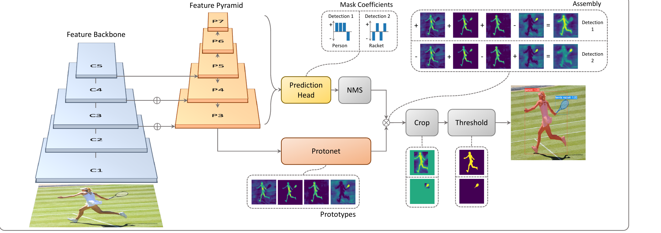
Fig. 2 (paper): backbone + FPN feed two parallel branches — Protonet (bottom) produces $k$ image-sized prototype masks, the Prediction Head (top) produces per-anchor mask coefficients alongside class and box. After NMS, surviving detections combine their coefficients with the prototypes and are cropped to the predicted box.

Core idea: decompose masks into prototypes × coefficients

Two-stage methods (Mask R-CNN, FCIS) depend on feature re-localization: an RPN proposes regions, feature maps are re-pooled into that region’s coordinate frame (RoIPool/RoIAlign), and only then does a small head predict a mask from the pooled features. This localization step is inherently sequential — the mask branch has to wait for region proposals — which makes it hard to parallelize and therefore hard to make fast.

YOLACT instead observes that instance segmentation can be split into two subtasks that are each easy for the network component best suited to them, and that neither one needs to know about individual instances up front:

1. Prototype generation (protonet): an FCN produces a fixed number $k$ of prototype masks over the entire image, independent of any instance and independent of the number of object categories (there can be more categories than prototypes).
2. Mask coefficient prediction: an extra branch on the detection head predicts, for each anchor, a $k$-vector of coefficients encoding how to combine the prototypes into that anchor’s instance mask.

For each detection surviving NMS, the final mask is a linear combination of the $k$ prototypes weighted by that instance’s coefficients, followed by a sigmoid and a crop to the predicted box. Because assembly is one matrix multiply, this adds only marginal computational overhead over the backbone detector — the paper reports the entire mask branch takes ~5 ms to evaluate.

Why this split works: convolutional (conv) layers are good at producing spatially coherent outputs but cannot easily produce one output “per instance” without knowing where instances are; fully-connected (fc) layers naturally produce one vector per instance (e.g. per anchor) but destroy spatial coherence. Protonet is all-conv and stays spatially coherent; the coefficient branch is a normal detection-head conv branch that still outputs one short vector per anchor, so no fc layer over spatial features is needed anywhere. An ablation (“fc-mask”: masks reshaped directly from an fc layer’s output, in the style of the original R-CNN mask branch) confirms the point — it collapses to 20.7 mAP, far below YOLACT’s 29.9.

Architecture

The detector backbone follows RetinaNet: ResNet-101 + FPN, base image size $550\times 550$ (no aspect-ratio preservation, for consistent per-image evaluation time), with $P_3$–$P_7$ (not $P_2$, unlike a stock FPN) and 3 anchors per cell with aspect ratios $[1,1/2,2]$ and scales $[24,48,96,192,384]$ across levels.

Protonet

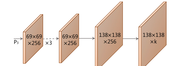
Fig. 3 (paper): protonet is a plain FCN — three $3\times 3$ convs, a $2\times$ bilinear upsample + conv to increase resolution before the final layer (important for small-object performance), and a final $1\times 1$ conv producing $k$ channels.

Protonet attaches to a single backbone feature level — the deepest, highest-resolution FPN level $P_3$, at $1/8$ input resolution — and outputs $k$ prototypes at $1/4$ resolution ($138\times 138$ for a $550\times 550$ input). Two design choices matter most: taking the protonet input from a deep backbone feature (more robust prototypes) while still upsampling before the last layer (better small-object performance, since predicting directly at $1/8$ resolution loses detail a $1/4$-resolution mask does not). The output has no bounding nonlinearity by default — ReLU rather than none, chosen for interpretability of the emergent prototypes, but the paper notes an unbounded output lets protonet produce large, confident activations for prototypes it’s sure about (e.g. obvious background).

Prediction head and mask coefficients

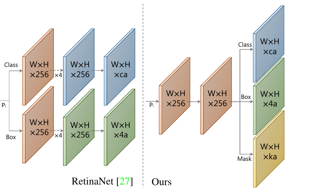
Fig. 4 (paper): compared to RetinaNet’s head (left), YOLACT’s own head (right) is shallower and adds a third parallel branch predicting $k$ mask coefficients per anchor, alongside the usual $c$ class scores and $4$ box regression values.

Where RetinaNet’s head produces $4+c$ values per anchor, YOLACT’s produces $4+c+k$: one shared $3\times 3$ conv followed by three parallel $3\times 3$ conv branches (class, box, mask coefficients). The mask-coefficient branch applies $\tanh$ to its $k$ outputs — critical, because it lets coefficients be negative, i.e. lets the network subtract a prototype’s contribution rather than only add it. Figure 5 of the paper shows this is exactly how overlapping same-class instances get separated: several prototypes learn to activate on one side of a soft, implicit spatial partition of the image, and an instance’s coefficient vector picks which side it’s on by adding one such prototype and subtracting another.

Mask assembly

$M=\sigma (P{C}^{\mathsf{T}})$

where $P\in {\mathbb{R}}^{h\times w\times k}$ is the matrix of prototype masks and $C\in {\mathbb{R}}^{n\times k}$ is the matrix of mask coefficients for the $n$ instances surviving NMS and score thresholding — a single matrix multiplication followed by a sigmoid, GPU-accelerated and with no further per-instance computation. Masks are then cropped to the predicted bounding box at evaluation time (cropped to the ground-truth box during training, with the mask loss divided by GT box area to preserve gradient signal for small objects).

Where translation variance comes from

A subtlety the paper is explicit about: instance segmentation needs translation variance (the same local pattern must produce a different mask depending on where in the image it sits, so distinct instances of the same appearance get distinct masks), but plain FCNs are largely translation invariant. FCIS and Mask R-CNN inject translation variance explicitly — directional maps, position-sensitive pooling, or simply moving the mask branch into the second (region-relative) stage. YOLACT adds only the minimal amount needed — cropping the final mask to the predicted box — and finds empirically that the network learns to localize instances mostly on its own, without cropping, for medium/large objects. This happens because modern FCNs like ResNet are not perfectly translation-invariant in practice: the zero-padding at every layer lets the network infer how far a given activation is from the image border, and through many stacked layers this leaks in enough positional information for protonet’s prototypes to specialize into implicit spatial partitions (Figure 5), directional maps, and one prototype that just segments “the ground.”

Fast NMS

Standard NMS is sequential: sort detections per class by confidence, then iterate, removing lower-scoring boxes overlapping a kept box above an IoU threshold. This sequential dependency is a hard floor on speed at real-time frame rates (a 10 ms improvement matters far more at 30 FPS than at 5 FPS). Fast NMS relaxes this: compute the $c\times n\times n$ pairwise IoU matrix for the top-$n$ per-class detections, zero out the lower triangle, take the column-wise max to get, for each detection, the highest IoU with any higher-scoring detection, and threshold that column-max vector — all as ordinary batched matrix operations with no recursion. The relaxation lets an already-removed detection still suppress others (impossible in standard NMS), which very occasionally removes slightly too many boxes; in practice this costs 0.1 mAP for an 11.8 ms speedup over a Cython NMS implementation (15.0 ms over Mask R-CNN’s CUDA NMS, for 0.3 mAP).

Auxiliary training-only losses

Two losses that cost nothing at inference (the modules that produce them are not run at test time), used purely to enrich the features the backbone learns during training:

• Semantic segmentation loss: a $1\times 1$ conv attached directly to $P_3$ predicts $c$ output channels with sigmoid (not softmax — a pixel can belong to more than one ground-truth instance’s class), trained with the instance annotations rasterized as a segmentation target. +0.4 mAP.
• The three total losses at inference-relevant training time are classification $L_{cls}$, box regression $L_{box}$ and mask loss $L_{mask}$ (pixel-wise binary cross-entropy between the assembled mask $M$ and ground truth $M_{gt}$), weighted $1:1.5:6.125$.

Hyperparameters

• Backbone: ResNet-101 + FPN (also evaluated: ResNet-50, DarkNet-53), ImageNet-pretrained.
• Image size: $550\times 550$ base (YOLACT-550); also trained at $400\times 400$ and $700\times 700$, with anchor scales adjusted by $s_x=s_{550}/550\cdot x$.
• Prototypes: $k=32$ (chosen as the accuracy/speed sweet spot; performance is stable down to $k=32$, and $k=64$–$256$ gives at most marginal AP${}_{95}$ gains).
• Optimizer: SGD, batch size 8 on one GPU, 800k iterations, initial LR $10^{-3}$, divided by 10 at iterations 280k/600k/700k/750k, momentum 0.9, weight decay $5\times 10^{-4}$.
• Data augmentation: same as SSD.
• Loss weights: $L_{cls}:L_{box}:L_{mask}=1:1.5:6.125$.
• Anchors: aspect ratios $[1,1/2,2]$, scales $[24,48,96,192,384]$ across $P_3$–$P_7$ (COCO); scales $\times 4/3$ for Pascal SBD, where objects tend to be larger.
• Positive/negative sampling: OHEM with a 3:1 negative:positive ratio; softmax cross-entropy for classification (not focal loss — found not viable in this setting, unlike RetinaNet).
• Training time: 4–6 days on one Titan Xp for COCO; under 1 day for Pascal.

Results

On COCO test-dev, single-model, no test-time augmentation:

Method	Backbone	FPS	AP	AP${}_{50}$	AP${}_{75}$	AP${}_S$	AP${}_M$	AP${}_L$
Mask R-CNN	R-101-FPN	8.6	35.7	58.0	37.8	15.5	38.1	52.4
MS R-CNN	R-101-FPN	8.6	38.3	58.8	41.5	17.8	40.4	54.4
FCIS	R-101-C5	6.6	29.5	51.5	30.2	8.0	31.0	49.7
YOLACT-550	R-101-FPN	33.5	29.8	48.5	31.2	9.9	31.3	47.1
YOLACT-400	R-101-FPN	45.3	24.9	42.0	25.4	5.0	25.3	45.0
YOLACT-700	R-101-FPN	23.4	31.2	50.6	32.8	12.1	33.3	47.1
YOLACT-550, R-50	R-50-FPN	40.7	28.2	46.6	29.2	9.2	27.9	45.5
YOLACT-550, D-53	D-53-FPN	40.7	28.4	46.7	30.0	9.5	29.6	45.5

3.8× the speed of the previous fastest instance segmentation method, at a real, if unglamorous, AP cost. Mask quality is a different story: because YOLACT’s masks come directly from full-image-resolution prototypes rather than a re-pooled RoI, at the 95% IoU threshold YOLACT’s base model scores 1.6 AP against Mask R-CNN’s 1.3, i.e. its masks are qualitatively better at high overlap despite being worse on average AP — RoI repooling in Mask R-CNN provably discards boundary precision. YOLACT masks are also more temporally stable on video despite training on static images only, because the mask branch does not depend on a per-frame region proposal the way two-stage methods do.

Limitations

The paper is explicit that YOLACT trades overall accuracy for speed and identifies two systematic, architecture-specific error modes, on top of ordinary detector mistakes (misclassification, box misalignment):

• Localization failure: when several objects cluster tightly in one spot, the network can fail to localize each in its own prototype combination and instead produce something closer to a single foreground blob spanning the group.
• Leakage: because masks are cropped to the box only after assembly, the assembly itself has no incentive to suppress activation outside an instance’s own box. If the predicted box is too big, or a far-away instance of the same or a different class overlaps the prototype’s activation, its mask can bleed into a neighboring instance’s crop.

Both effects are secondary to detector quality, not mask quality: the paper measures only a 2.5 mAP box→mask gap for YOLACT-550 (32.3 box AP vs. 29.8 mask AP) — almost identical to Mask R-CNN’s own 2.5-point gap (38.2 → 35.7) — implying the ~6 mAP overall deficit against Mask R-CNN is explained by YOLACT’s weaker one-stage detector, not by its prototype-based approach to producing masks.

Legacy: YOLOv8-seg

YOLOv8’s segmentation head (-seg checkpoints) reuses YOLACT’s prototype + coefficient decomposition essentially unchanged, grafted onto YOLOv8’s anchor-free, decoupled detection head instead of RetinaNet-style anchors: protonet still produces a fixed bank of prototype masks from a backbone feature map, and each detected instance still gets a coefficient vector combined with the prototypes via the same $M=\sigma (P{C}^{\mathsf{T}})$ assembly. The main practical difference is upstream of the mask head — anchor-free assignment replaces anchor-based coefficient prediction — not in how a mask is produced from prototypes.

See also

• YOLOv8 — the anchor-free detector whose -seg variant inherits this prototype-based mask head almost unchanged
• Mask R-CNN — the RoIAlign + per-class FCN mask head this architecture was designed to avoid the sequential cost of
• SOLOv2 — a box-free alternative that also decouples mask generation into two components (feature map + per-instance kernel) but conditions the kernel dynamically on backbone features rather than a fixed prototype dictionary
• Segmentation Head Comparison — this architecture placed side by side with Mask R-CNN’s, SOLOv2’s, DETR’s and Mask2Former’s mask heads
• Task-Aligned-Assignment — the label assignment YOLOv8 uses for the detection side of its head that YOLACT’s coefficient branch sits on top of