HSNet

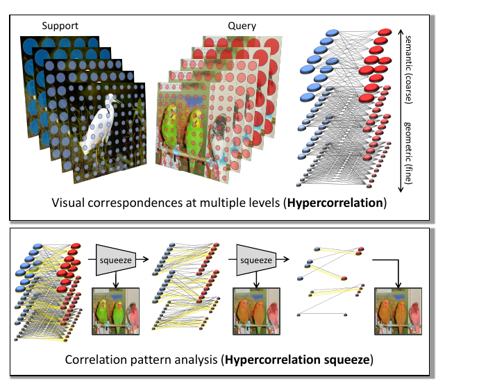
HSNet (Hypercorrelation Squeeze Networks) is a few-shot semantic segmentation model that treats the task as analysing dense feature correspondences rather than as matching prototypes.

• Paper: Juhong Min, Dahyun Kang, Minsu Cho (POSTECH), Hypercorrelation Squeeze for Few-Shot Segmentation, ICCV 2021, arXiv:2104.01538.
• Core idea: build a pyramid of 4D correlation tensors, a hypercorrelation, from every intermediate convolutional layer of a frozen backbone, and squeeze it down to a segmentation mask with deeply stacked 4D convolutions.
• Center-pivot 4D convolution: the second contribution; a weight-sparsified 4D kernel that decomposes into two 2D convolutions.
• Cost and result: cuts the model to 2.6M learnable parameters and 25.5 ms per episode while improving accuracy over dense 4D kernels.

Problem setup

Few-shot semantic segmentation segments a target object in a query image given only a few annotated support images of the same class. Training and test sets ${\mathcal{D}}_{\text{train}},{\mathcal{D}}_{\text{test}}$ are disjoint with respect to object classes, and training is episodic: each episode samples a support set $\mathcal{S}=(I^{\text{s}},{\mathbf{M}}^{\text{s}})$ and a query set $\mathcal{Q}=(I^{\text{q}},{\mathbf{M}}^{\text{q}})$, and the model learns a mapping $(I^{\text{s}},{\mathbf{M}}^{\text{s}},I^{\text{q}})\mapsto {\mathbf{M}}^{\text{q}}$. At test time the learned mapping is applied to novel classes with no further optimization.

The dominant prior paradigm is prototypical: masked average pooling collapses the support foreground into one (or a few) global vectors, which are then compared against query features. That discards spatial structure. HSNet instead keeps all pairwise support-query matches and learns to read the geometric patterns in them — importing two ideas from the semantic-correspondence literature (multi-level features, and 4D convolutions for neighbourhood consensus) into few-shot segmentation.

Architecture

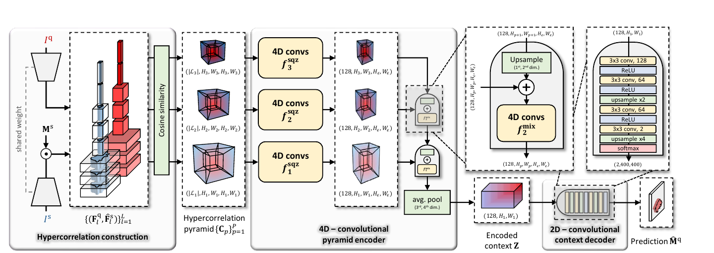
Three stages: hypercorrelation construction, a 4D-convolutional pyramid encoder, and a 2D-convolutional context decoder.

Hypercorrelation construction

Query and support images $I^{\text{q}},I^{\text{s}}\in {\mathbb{R}}^{3\times H\times W}$ go through the same frozen backbone, producing $L$ pairs of intermediate feature maps $\{({\mathbf{F}}_l^{\text{q}},{\mathbf{F}}_l^{\text{s}}){\}}_{l=1}^L$ — $L=7$ for VGG16, $13$ for ResNet50, $30$ for ResNet101, i.e. essentially every conv layer of the last blocks, not just the final one.

Each support feature map is masked to discard background activations:

${\hat{\mathbf{F}}}_l^{\text{s}}={\mathbf{F}}_l^{\text{s}}\odot {\zeta }_l({\mathbf{M}}^{\text{s}}),$

where $\odot$ is the Hadamard product and ${\zeta }_l$ bilinearly interpolates the mask to layer $l$‘s spatial size and expands it along channels.

Each layer then yields a 4D correlation tensor ${\hat{\mathbf{C}}}_l\in {\mathbb{R}}^{H_l\times W_l\times H_l\times W_l}$ by cosine similarity between every query position ${\mathbf{x}}^{\text{q}}$ and every support position ${\mathbf{x}}^{\text{s}}$:

${\hat{\mathbf{C}}}_l({\mathbf{x}}^{\text{q}},{\mathbf{x}}^{\text{s}})=\mathrm{ReLU}\left(\frac{{\mathbf{F}}_l^{\text{q}}({\mathbf{x}}^{\text{q}})\cdot {\hat{\mathbf{F}}}_l^{\text{s}}({\mathbf{x}}^{\text{s}})}{\Vert {\mathbf{F}}_l^{\text{q}}({\mathbf{x}}^{\text{q}})\Vert \Vert {\hat{\mathbf{F}}}_l^{\text{s}}({\mathbf{x}}^{\text{s}})\Vert }\right),$

the ReLU suppressing noisy negative scores. Tensors sharing a spatial resolution are concatenated along a new channel dimension into a hypercorrelation ${\mathbf{C}}_p\in {\mathbb{R}}^{|{\mathcal{L}}_p|\times H_p\times W_p\times H_p\times W_p}$ at pyramidal layer $p$. With $P=3$ pyramid levels for all backbones, this gives the pyramid $\mathcal{C}=\{{\mathbf{C}}_p{\}}_{p=1}^P$ at resolutions $50,25,13$ (ResNet) or $50,25,12$ (VGG16). Note the correlation itself is parameter-free — it is a similarity, not a learned matching head, exactly as in PerSAM’s location prior, only computed densely at every level instead of pooled.

4D-convolutional pyramid encoder

Two building-block types, each three sequences of multi-channel 4D convolution → group normalization → ReLU:

• Squeezing block $f_p^{\text{sqz}}$: strides periodically squeeze the support spatial dimensions $(H_p,W_p)\to (H_{ϵ},W_{ϵ})$ (down to $2\times 2$ in practice) while the query dimensions are preserved:
  $f_p^{\text{sqz}}:{\mathbb{R}}^{|{\mathcal{L}}_p|\times H_p\times W_p\times H_p\times W_p}\to {\mathbb{R}}^{128\times H_p\times W_p\times H_{ϵ}\times W_{ϵ}}.$
• Mixing block $f_p^{\text{mix}}$: FPN-style top-down propagation — the output of level $p+1$ is upsampled by 2 along the query dimensions and added element-wise to level $p$‘s output, then processed by further 4D convs.

After iterative top-down mixing, the lowest block’s output ${\mathbf{C}}_1^{\text{mix}}$ is average-pooled over its support dimensions, giving a 2D context $\mathbf{Z}\in {\mathbb{R}}^{128\times H_1\times W_1}$ that condenses the whole hypercorrelation. This is the “coarse-to-fine squeeze”: high-level semantic evidence from the deep, low-resolution correlations is propagated down into the fine geometric correlations before collapsing.

2D-convolutional context decoder

A small stack of 2D convs, ReLU and upsampling (3x3 conv 128 → ReLU → 3x3 conv 64 → ReLU → upsample ×2 → 3x3 conv 64 → ReLU → 3x3 conv 2 → upsample ×4 → softmax), producing a two-channel map ${\tilde{\mathbf{M}}}^{\text{q}}\in [0,1{]}^{2\times H\times W}$ of foreground/background probabilities. 259K parameters, identical for all backbones.

Center-pivot 4D convolution

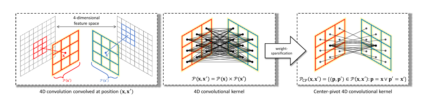
A 4D convolution with kernel $k\in {\mathbb{R}}^{\hat{k}\times \hat{k}\times \hat{k}\times \hat{k}}$ on a correlation tensor $c\in {\mathbb{R}}^{H\times W\times H\times W}$ at position $(\mathbf{x},{\mathbf{x}}^{\prime })\in {\mathbb{R}}^4$ is

$(c\ast k)(\mathbf{x},{\mathbf{x}}^{\prime })={\sum }_{(\mathbf{p},{\mathbf{p}}^{\prime })\in \mathcal{P}(\mathbf{x},{\mathbf{x}}^{\prime })}c(\mathbf{p},{\mathbf{p}}^{\prime })k(\mathbf{p}-\mathbf{x},{\mathbf{p}}^{\prime }-{\mathbf{x}}^{\prime }),$

with the 4D neighbourhood the Cartesian product $\mathcal{P}(\mathbf{x},{\mathbf{x}}^{\prime })=\mathcal{P}(\mathbf{x})\times \mathcal{P}({\mathbf{x}}^{\prime })$ — hence ${\hat{k}}^4$ weights and quadratic complexity in the feature-map size. Two problems follow. Cost: this is why prior correspondence work could afford only a few 4D layers. Over-parameterization: a single activation is touched a number of times exponential in the dimensionality, so unreliable large-magnitude activations at insignificant 4D positions inject noise.

HSNet’s answer is weight sparsification: keep only the neighbours that pivot on one of the two 2D centers $\mathbf{x}$ or ${\mathbf{x}}^{\prime }$,

${\mathcal{P}}_c(\mathbf{x},{\mathbf{x}}^{\prime })=\{(\mathbf{p},{\mathbf{p}}^{\prime })\in \mathcal{P}(\mathbf{x},{\mathbf{x}}^{\prime }):\mathbf{p}=\mathbf{x}\},{\mathcal{P}}_{c^{\prime }}(\mathbf{x},{\mathbf{x}}^{\prime })=\{(\mathbf{p},{\mathbf{p}}^{\prime })\in \mathcal{P}(\mathbf{x},{\mathbf{x}}^{\prime }):{\mathbf{p}}^{\prime }={\mathbf{x}}^{\prime }\},$

and ${\mathcal{P}}_{\text{CP}}={\mathcal{P}}_c\cup {\mathcal{P}}_{c^{\prime }}$. The resulting center-pivot (CP) 4D convolution is a union of two separate 4D convolutions, $(c\ast k_{\text{CP}})=(c\ast k_c)+(c\ast k_{c^{\prime }})$, which — because each collapses onto a fixed 2D slice of the tensor — reduces exactly to two 2D convolutions:

$(c\ast k_{\text{CP}})(\mathbf{x},{\mathbf{x}}^{\prime })={\sum }_{{\mathbf{p}}^{\prime }\in \mathcal{P}({\mathbf{x}}^{\prime })}c(\mathbf{x},{\mathbf{p}}^{\prime })k_c^{\text{2D}}({\mathbf{p}}^{\prime }-{\mathbf{x}}^{\prime })+{\sum }_{\mathbf{p}\in \mathcal{P}(\mathbf{x})}c(\mathbf{p},{\mathbf{x}}^{\prime })k_{c^{\prime }}^{\text{2D}}(\mathbf{p}-\mathbf{x}),$

with $k_c^{\text{2D}}=k(0,:)\in {\mathbb{R}}^{\hat{k}\times \hat{k}}$ and $k_{c^{\prime }}^{\text{2D}}=k(:,0)\in {\mathbb{R}}^{\hat{k}\times \hat{k}}$. Weights drop from ${\hat{k}}^4$ to $2{\hat{k}}^2$ and complexity becomes linear, which is what makes deeply stacked 4D convolutions affordable at all. The full derivation is Appendix A of the paper.

Unlike the spatially separable 4D kernel of Yang & Ramanan, which needs auxiliary transformation layers with batch normalization for numerical stability, the CP decomposition is a sum of two independent 2D convolutions and needs none — hence half the parameters and half the latency.

Training and $K$-shot inference

The backbone is frozen throughout — only the encoder and decoder are learned (2.6M parameters for every backbone). The network is optimized with the mean of the cross-entropy loss between the two-channel prediction ${\tilde{\mathbf{M}}}^{\text{q}}$ and the ground truth ${\mathbf{M}}^{\text{q}}$ over all pixel locations; at test time the per-pixel argmax gives ${\hat{\mathbf{M}}}^{\text{q}}\in \{0,1{\}}^{H\times W}$.

$K$-shot inference needs no architectural change: run $K$ forward passes to get $\{{\bar{\mathbf{M}}}_k^{\text{q}}{\}}_{k=1}^K$, sum the predictions at every pixel, divide by the maximum voting score, and threshold at $\tau =0.5$ for the foreground.

Freezing the backbone is not merely an efficiency choice. The ablation on fine-tuning (Fig. 9) shows a fine-tuned backbone — even with its learning rate set 100× lower — rapidly overfits the training folds and loses validation mIoU, while the frozen model keeps the generic ImageNet representation and generalizes to novel classes. The claim is that in the few-shot regime one should learn feature correlations, not features.

Hyperparameters

Setting	Value
Backbones	VGG16, ResNet50, ResNet101 (ImageNet-pretrained, frozen)
Feature extraction (VGG16)	after every conv layer in conv4_x–conv5_x, plus after the last maxpool; $L=7$
Feature extraction (ResNet)	end of each bottleneck before the ReLU, conv3_x–conv5_x; $L=13$ (R50), $L=30$ (R101)
Pyramid levels	$P=3$ for all backbones
Input resolution	$400\times 400$ ($H=W=400$), support and query alike
Correlation resolutions	$(H_1,W_1)=50$, $(H_2,W_2)=25$, $(H_3,W_3)=13$ (ResNet) / $12$ (VGG16)
Squeezed support size	$(H_{ϵ},W_{ϵ})=2\times 2$
Encoder channels	128
4D convs per building block	3 (accuracy saturates beyond this)
Normalization	group norm, $g=4$ groups
Optimizer	Adam, learning rate $1\times 10^{-3}$
Batch size	20 (PASCAL-5${}^i$), 40 (COCO-20${}^i$), 20 (FSS-1000)
Framework	PyTorch
$K$-shot voting threshold	$\tau =0.5$
Data augmentation	none
Learnable parameters	2.6M for every backbone (decoder 259K; squeezing blocks ~168–203K each; mixing blocks 886K each)
Evaluation protocol	4-fold cross-validation, 1,000 randomly sampled episodes per target fold

The paper does not state a number of training epochs (it trains to validation-mIoU convergence; the learning curves in Fig. 9 run to roughly 100 epochs on PASCAL-5${}^i$).

Results

Metrics are mean IoU (averaged over the classes of a fold) and foreground-background IoU, $\text{FB-IoU}=\frac{1}{2}({\text{IoU}}_{\text{F}}+{\text{IoU}}_{\text{B}})$; the paper focuses on mIoU as the better indicator of generalization.

PASCAL-5${}^i$ (mIoU averaged over the 4 folds):

Backbone	1-shot mIoU	1-shot FB-IoU	5-shot mIoU	5-shot FB-IoU	Params
VGG16	59.7	73.4	64.1	76.6	2.6M
ResNet50	64.0	76.7	69.5	80.6	2.6M
ResNet101	66.2	77.6	70.4	80.6	2.6M
ResNet101, no support masking	61.5	72.5	63.7	73.8	2.6M

With ResNet101 this is +6.1%p (1-shot) and +4.8%p (5-shot) mIoU over PFENet, with the fewest learnable parameters of any compared method (PFENet 10.8M, RePRI 46.7M, FWB 43.0M, OSLSM 276.7M).

COCO-20${}^i$:

Backbone	1-shot mIoU	1-shot FB-IoU	5-shot mIoU	5-shot FB-IoU
ResNet50	39.2	68.2	46.9	70.7
ResNet101	41.2	69.1	47.1	72.4

+2.7%p (1-shot) and +6.8%p (5-shot) over PFENet with ResNet101.

FSS-1000 (mIoU): VGG16 82.3 / 85.8, ResNet50 85.5 / 87.8, ResNet101 86.5 / 88.5 (1-shot / 5-shot) — state of the art on all three benchmarks.

Larger $K$ (ResNet50, PASCAL-5${}^i$ / COCO-20${}^i$): 64.0 / 39.2 at $K=1$, 69.5 / 46.9 at $K=5$, 70.6 / 48.7 at $K=10$, i.e. +2.5%p and +4.6%p over the previous best at 10-shot.

Efficiency

Comparison of the three 4D kernels (ResNet101, PASCAL-5${}^i$; timings on an Intel i7-7820X and an NVIDIA Titan-XP):

Kernel	1-shot mIoU	5-shot mIoU	Params	Time / episode	Memory	FLOPs
Original dense 4D	64.9	70.1	11.3M	512.17 ms	4.12 GB	702.35 G
Spatially separable 4D	65.9	70.2	4.4M	28.48 ms	1.50 GB	28.40 G
Center-pivot 4D (ours)	66.2	70.4	2.6M	25.51 ms	1.39 GB	20.56 G

A 20× speed-up and 34× FLOP reduction over the dense kernel, with higher accuracy — direct evidence that most weights in a high-dimensional kernel are not merely redundant but actively harmful.

Ablations

• Multi-level vs. single-level correlation (ResNet101, PASCAL-5${}^i$ 1-shot mIoU): ${\mathbf{C}}_p^{\text{shallow}}$ (a single shallowest correlation) 59.1, ${\mathbf{C}}_p^{\text{deep}}$ (single deepest) 61.7, full multi-channel ${\mathbf{C}}_p$ 66.2. So +4.5%p from stacking all intermediate layers, and the shallow-vs-deep gap confirms that reliable features live in deeper layers.
• Pyramid layers: ${\mathcal{C}}^{(3)}$ (deepest level only) 55.5, ${\mathcal{C}}^{(2:3)}$ 63.9, full $\mathcal{C}$ 66.2 (1-shot). Without the geometric (fine) levels the model gives only coarse localization and cannot refine boundaries; the intermediate level $p=2$ is especially important.
• Depth of building blocks: accuracy improves up to three 4D conv layers per block, then saturates.
• Support masking: removing Eqn. 1 entirely (a setting close to co-segmentation) still gives 61.5 mIoU 1-shot with ResNet101, +1.4%p over the previous best masked method (and 63.7 at 5-shot, rivalling it) — the model can identify the common instance across two images without being told where it is in the support.
• Domain shift (train on COCO-20${}^i$, test on PASCAL-5${}^i$, disjoint classes, no data augmentation): HSNet-R50 61.6 (1-shot) / 68.7 (5-shot), HSNet-R101 64.1 / 70.3, versus RePRI 63.2 / 67.7 with 46.7M parameters and flip augmentation, and PFENet 61.1 / 63.4 with flip/rotate/crop.
• ignore_label: some prior methods do not use PASCAL’s ambiguous-boundary ignore label. Evaluated without it too, HSNet-R50 still gets 59.1 (1-shot) / 64.2 (5-shot) mIoU, +2.8%p / +5.4%p over the best of those methods.

Limitations

• Quadratic correlation cost. The CP kernel makes the convolutions linear, but the hypercorrelation tensor itself is still $H_p{W}_p{H}_p{W}_p$ per level — memory grows quadratically with feature-map resolution, which caps the input at $400\times 400$ and the finest correlation at $50\times 50$.
• Frozen backbone caps the representation. Everything downstream depends on ImageNet features that were never adapted to the task; fine-tuning them overfits, so the ceiling is whatever correspondence signal those features already contain.
• Failure modes (Fig. A11): severe occlusion, large intra-class variance between support and query, and extremely tiny objects in either image cause localization failures.
• No data augmentation is used, and the paper notes domain-shift robustness “may further increase” with the augmentations used by competitors — the reported numbers are therefore not the ceiling.
• Support masking is at feature resolution. The mask is bilinearly downsampled to each layer’s grid, so thin structures are lost before the correlation is even computed.
• The method solves a class-agnostic binary task per episode; multi-class segmentation requires one pass per class, and $K$-shot inference costs $K$ forward passes since aggregation happens at the prediction level, not in the feature space.

See also

• PerSAM — the same idea of dense cosine-similarity matching against a masked reference feature map, but training-free and on top of a frozen SAM rather than feeding a learned 4D-conv encoder.
• SAM — promptable segmentation from a very different angle: instead of learning to match one support example, train on 1.1B masks so a click suffices.
• SAM3 — promptable concept segmentation, including with exemplar images; the modern, foundation-model answer to the problem HSNet attacks with correspondence.
• Your ViT is Secretly an Image Segmentation Model — the opposite architectural bet: strip the specialized segmentation machinery and let a large pre-trained ViT do the work.
• Implementing Research Papers — HSNet’s episodic 4-fold protocol and 1,000-episode sampling are exactly the kind of evaluation detail that decides whether a reproduction matches.