SAM (Segment Anything Model)

SAM is a promptable image segmentation model.

Paper: Kirillov, Mintun, Ravi, Mao, Rolland, Gustafson, Xiao, Whitehead, Berg, Lo, Dollár, Girshick (Meta AI Research, FAIR), Segment Anything, ICCV 2023, arXiv:2304.02643.
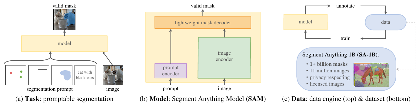
Ambition: not a single model but a foundation model for segmentation, delivered as three interlocking pieces.
Task: a new task, promptable segmentation.
Model: SAM, fast enough to be prompted interactively.
Data engine: used the model in the loop to build SA-1B, 1.1B masks over 11M images, ~400× more masks than any prior segmentation dataset.

SAM task, model and data

The promptable segmentation task

The task is transplanted from NLP: given an image and a prompt, return a valid segmentation mask. A prompt is anything that indicates what to segment — a set of foreground/background points, a rough box, a coarse mask, or free-form text.

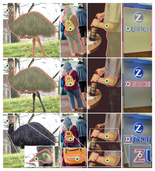
The word valid is doing the work. A prompt can be ambiguous: a point on a shirt may refer to the shirt or to the person wearing it. The requirement is only that the output be a reasonable mask for at least one of the plausible objects — analogous to expecting a language model to give a coherent response to an ambiguous prompt.

This choice is what makes the task usable as both (a) a pre-training objective (simulate a sequence of prompts per training sample, compare against ground truth) and (b) a general interface for zero-shot transfer: downstream tasks are solved by prompt engineering rather than fine-tuning. Instance segmentation, for instance, becomes “run a box detector, feed its boxes to SAM as prompts”.

Three valid masks from one ambiguous point prompt

Architecture

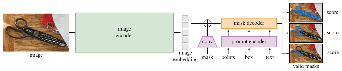
SAM overview: image encoder, prompt encoder, mask decoder

Real-time interactive use imposes the architecture. SAM splits into a heavyweight image encoder that runs once per image and a fast prompt encoder + mask decoder that run once per prompt, so the expensive image embedding is computed once and amortized across arbitrarily many prompts. Prompt encoder and decoder run in ~50 ms in a browser on CPU given a precomputed embedding.

Image encoder

An MAE pre-trained ViT-H/16, minimally adapted for high resolution: $14 \times 14$ windowed attention with four equally-spaced global attention blocks. Input images are rescaled and padded to $1024 \times 1024$ , giving a $16 \times$ -downscaled $64 \times 64$ embedding. Channels are reduced to 256 by a $1 \times 1$ convolution followed by a $3 \times 3$ convolution, each followed by layer normalization.

Prompt encoder

Two families of prompts:

Sparse (points, boxes, text) → 256-dimensional embeddings.
- A point is a positional encoding of its location summed with one of two learned embeddings marking foreground or background.
- A box is a pair of embeddings: the positional encoding of its top-left corner plus a learned “top-left corner” embedding, and the same for the bottom-right.
- Text is embedded with the off-the-shelf CLIP text encoder.
Dense (masks) → input at $4 \times$ lower resolution than the image, downscaled another $4 \times$ by two stride-2 $2 \times 2$ convolutions (output channels 4 and 16, GELU + layer norm between), then a $1 \times 1$ convolution to 256 channels, and added element-wise to the image embedding. If no mask prompt is given, a learned “no mask” embedding is added at every location instead.

Mask decoder

Lightweight mask decoder

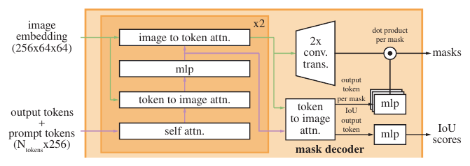
A modified two-layer Transformer decoder that updates both the prompt tokens and the image embedding. A learned output token (analogous to BERT’s [class] token) is prepended to the prompt embeddings. Each decoder layer performs four steps:

self-attention over the tokens,
cross-attention tokens → image embedding (tokens as queries),
a point-wise MLP updating each token,
cross-attention image embedding → tokens (image as queries), which writes prompt information back into the image embedding.

Each block has a residual connection, layer normalization, and dropout of 0.1. Positional encodings are re-added to the image embedding at every attention layer, and the entire original prompt token (positional encoding included) is re-added to the updated tokens — a strong dependence on both geometric location and prompt type.

After the decoder, the image embedding is upscaled $4 \times$ with two transposed convolutions (output channels 64 and 32, GELU, layer norm), the tokens attend to it once more, and the updated output token goes through a 3-layer MLP. The mask is then a spatially point-wise dot product between the upscaled embedding and the MLP’s output — i.e. a dynamic linear classifier over image locations. Transformer embedding dimension is 256 (reduced to 128 inside cross-attention for queries/keys/values), MLP internal dimension 2048, 8 heads throughout.

Resolving ambiguity

With a single output the model would learn to average over the valid masks of an ambiguous prompt. Instead SAM uses several output tokens and predicts 3 masks simultaneously — empirically enough, since nested masks are usually at most three deep (whole, part, subpart). During training the loss is computed against all three but only the minimum-loss mask is backpropagated. A small head on an additional output token predicts each mask’s IoU with the object it covers, which is used to rank the masks and expose a confidence score.

Ambiguity is much rarer with multiple prompts, so a fourth output token is added and used only when more than one prompt is given; it is never returned for a single prompt.

Losses and training

Mask supervision is a linear combination of focal loss and dice loss in a 20:1 ratio, with auxiliary deep supervision after each decoder layer. The IoU prediction head is trained with MSE between predicted IoU and the actual IoU of the predicted mask against ground truth, added to the mask loss with a scaling factor of 1.0.

Training simulates an interactive setup. The first prompt is, with equal probability, a foreground point sampled uniformly from the ground truth mask or that mask’s bounding box with per-coordinate Gaussian noise (std = 10% of the box side length, capped at 20 pixels). Subsequent points are sampled uniformly from the error region between the previous prediction and ground truth, labelled foreground or background depending on whether that region is a false negative or false positive. The previous iteration’s unthresholded mask logits are supplied as an additional (dense) prompt to carry maximal information forward; when multiple masks are returned, the one with highest predicted IoU is passed on.

There are 11 iterations total: the initial prompt, 8 iteratively sampled points, and 2 iterations with no new external information (one inserted randomly, one always at the end) so the model learns to refine its own predictions. This is affordable only because the decoder is <1% of the image encoder’s compute.

Hyperparameters

Transcribed from §A of the paper (default SAM / ViT-H recipe):


Optimizer	AdamW ( $β_{1} = 0.9$ , $β_{2} = 0.999$ )
LR warmup	linear, 250 iterations
Initial LR (after warmup)	$8 \times 1 0^{- 4}$
LR schedule	step-wise decay; $\div 10$ at 60k and again at 86,666 iterations
Iterations	90k (~2 SA-1B epochs)
Batch size	256 images
Weight decay ( $w d$ )	0.1
Drop path ( $d p$ )	0.4
Layer-wise LR decay ( $l d$ )	0.8
Data augmentation	none
Initialization	MAE pre-trained ViT-H
Hardware	256 GPUs; up to 64 randomly sampled masks per GPU
Input resolution	$1024 \times 1024$
Mask loss	20:1 focal : dice
Decoder dropout	0.1

Deviations: ViT-B and ViT-L were trained for 180k iterations, batch size 128, on 128 GPUs, with $l r = 8 \times 1 0^{- 4} /4 \times 1 0^{- 4}$ , $l d = 0.6/0.8$ , $w d = 0.1$ , $d p = 0.6/0.4$ respectively. Training on data-engine stages one and two only used large-scale jitter with scale range $[0.1, 2.0]$ , since data is more limited there. SA-1B masks covering more than 90% of the image are filtered out.

The dedicated automatic mask generation variant was trained differently again: 177,656 iterations, large-scale jitter, point and mask prompts only (no boxes), 4 points sampled per mask instead of 9, and a 3-layer mask decoder.

Data engine

Masks are not abundant on the internet, so the dataset was co-developed with the model in three stages:

Assisted-manual. Annotators click foreground/background points in a browser tool powered by SAM (real-time thanks to precomputed embeddings), refining with brush and eraser. No semantic constraints — both “stuff” and “things”, labelled in order of prominence, moving on after 30 s per mask. SAM was retrained 6 times as data accumulated and the encoder scaled ViT-B → ViT-H. Average annotation time fell 34 s → 14 s (6.5× faster than COCO annotation, only 2× slower than bounding-box labelling with extreme points); masks per image rose 20 → 44. 4.3M masks from 120k images.
Semi-automatic. To increase mask diversity, confident masks were pre-filled automatically (detected by running a bounding-box detector on first-stage masks under a generic “object” category) and annotators labelled only the remaining unannotated objects. Time per mask went back up to 34 s (harder objects); masks per image 44 → 72. Model retrained 5 times. +5.9M masks in 180k images (10.2M total).
Fully automatic. SAM is prompted with a regular $32 \times 32$ grid of points; for each point the ambiguity-aware model returns subpart/part/whole candidates. The IoU head selects confident masks; stable masks are kept (thresholding the probability map at $0.5 - δ$ and $0.5 + δ$ must give similar masks); NMS removes duplicates; zoomed-in image crops improve small masks. Applied to all 11M images → 1.1B masks.

Automatic generation details

Masks come from a $32 \times 32$ grid on the full image plus 20 zoomed-in crops ( $2 \times 2$ and $4 \times 4$ overlapping windows, with $16 \times 16$ and $8 \times 8$ point grids). Greedy box-based NMS at threshold 0.7, applied first within each crop then across crops (ranking more-zoomed-in masks above less). Filters: predicted IoU threshold 88.0; stability — IoU between the masks thresholded at $- 1$ and $+ 1$ logits must be $\geq$ 95.0; masks covering $\geq$ 95% of the image are dropped. Postprocessing removes connected components under 100 px and fills holes under 100 px.

SA-1B

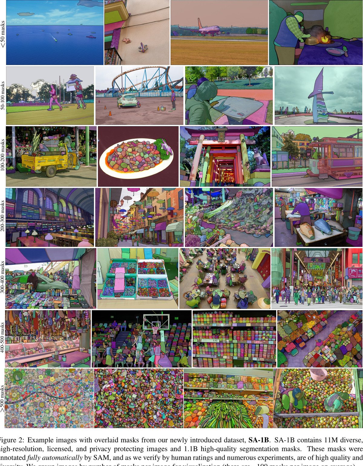
SA-1B examples grouped by masks per image

11M licensed, privacy-protecting images (3300×4950 px on average, released downsampled to 1500 px shortest side; faces and license plates blurred) and 1.1B masks, 99.1% of them fully automatic. On average ~100 masks per image — $36 \times$ more masks per image than Open Images, $11 \times$ more images and $400 \times$ more masks than the largest prior dataset.

Mask quality. 500 images (~50k masks) were re-annotated professionally: 94% of automatic/corrected pairs exceed 90% IoU (97% exceed 75%), against 85–91% IoU inter-annotator consistency reported in prior work. Because automatic masks proved this good, SA-1B ships only automatically generated masks. Ablations confirm training on automatic masks alone is within ~0.5 mIoU of using all data-engine data.

Zero-shot transfer results

Five tasks, four of which differ substantially from the training task and are reached purely by prompt engineering:

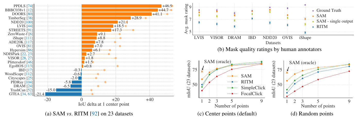
Point-to-mask evaluation on 23 datasets

Single-point valid mask (23-dataset suite). SAM beats the strongest interactive segmenter, RITM, on 16 of 23 datasets by up to ~47 IoU. With the “oracle” mask of its 3 predictions selected against ground truth, SAM wins on all 23 — the automatic-metric losses are an artifact of ambiguity, not quality. Human annotators rate SAM’s masks consistently higher than RITM’s (typically 7–9 on a 1–10 scale), including on datasets where SAM loses on mIoU. As the number of points grows 1 → 9, the gap to baselines closes.
Edge detection (BSDS500), by prompting a $16 \times 16$ point grid, NMS-ing redundant masks and Sobel-filtering the mask probability maps: ODS .768, OIS .786, AP .794, R50 .928 — beating HED (.788/.808/.840/.923) on recall and comfortably beating Canny/Felz-Hutt, while lagging supervised SOTA on precision because SAM predicts more edges than BSDS annotates.
Object proposals (LVIS v1, mask AR@1000): 59.3 overall vs. 63.0 for a supervised ViTDet-H “detector masquerading as proposal generator” baseline — but SAM wins on medium, large, rare and common objects (e.g. rare 65.8 vs. 58.3), losing only on small and frequent objects where ViTDet exploits LVIS-specific annotation biases.
Instance segmentation (prompt SAM with ViTDet’s boxes): COCO 46.5 AP vs. 51.0, LVIS 44.7 vs. 46.6. Lower AP, but human raters score SAM’s masks higher than ViTDet’s (8.1 vs. 7.9 on LVIS) — evidence ViTDet is fitting the ground truth’s biases rather than producing better boundaries.
Text-to-mask (proof of concept): during training, for each mask with area > $10 0^{2}$ , the CLIP image embedding is extracted and used as the first prompt; at inference CLIP’s text embedding is substituted, exploiting CLIP’s image–text alignment so that no text annotations are ever needed. Works for “a wheel” and even “beaver tooth grille”; failures are often fixed by adding one point prompt.

Ablations

Data engine, data scale and encoder scale ablations

Each data engine stage improves mIoU; but since automatic masks vastly outnumber the others, using automatic data only is nearly as good (~0.5 mIoU) and much simpler.
Data scale: 0.1M images degrades badly, but 1M images (~10% of SA-1B, ~100M masks) is comparable to the full 11M — a practical setting for most users.
Encoder scale: ViT-H improves substantially over ViT-B but only marginally over ViT-L. Further scaling does not look fruitful.

Limitations

Misses fine structures and sometimes hallucinates small disconnected components.
Boundaries are less crisp than computationally intensive “zoom-in” methods like FocalClick.
Dedicated interactive segmenters outperform SAM when many points are provided; SAM optimizes breadth, not the high-IoU regime.
Prompt encoder and decoder are real-time, but the heavy image encoder means the overall pipeline is not.
Text-to-mask is exploratory and not robust.
Unclear how to design prompts expressing semantics — SAM produces masks, not labels — and no simple prompt handles semantic/panoptic segmentation.

Responsible AI

SA-1B spans more countries with >1000 images than any prior dataset; the top three image-contributing countries are on different continents. Europe and Asia & Oceania and middle-income countries are over-represented relative to COCO/Open Images; Africa and low-income countries remain under-represented (0.9% of images) in all datasets, though even Africa has 28M masks — 10× the total mask count of any previous dataset. Measured on MIAP, SAM’s mIoU differences across perceived gender presentation, age group, and skin tone are mostly within overlapping 95% confidence intervals (only older vs. middle age differs). Segmenting clothing, however, shows a disjoint gap by perceived gender presentation at 1 point (masculine 81.0 vs. feminine 76.3), narrowing at 3 points.

Wiki

Explorer

SAM