DINO

DINO (DETR with Improved deNoising anchOr boxes) is an end-to-end object detector in the DETR line.

• Paper: Zhang, Li, Liu, Zhang, Su, Zhu, Ni and Shum (HKUST / Tsinghua / IDEA), DINO: DETR with Improved DeNoising Anchor Boxes for End-to-End Object Detection, ICLR 2023, arXiv:2203.03605.
• Not the other DINO: this is not the self-supervised-learning DINO from Meta (Emerging Properties in Self-Supervised Vision Transformers, arXiv:2104.14294) — the acronym is badly overloaded; this one is a detector and has nothing to do with self-distillation or ViT feature learning.
• Built from: the Deformable DETR backbone plus DAB-DETR’s anchor-box queries and DN-DETR’s denoising training.
• New ingredients: contrastive denoising training, mixed query selection for anchor initialization, and look forward twice for box refinement.
• ResNet-50 result: 49.4 AP in 12 epochs and 51.3 AP in 24 epochs on COCO val2017 with multi-scale features ($+6.0$ / $+2.7$ AP over the previous best DETR-like model).
• Headline result: with a SwinL backbone pre-trained on ImageNet-22K and detection pre-training on Objects365, 63.2 AP on val2017 and 63.3 AP on test-dev, the first time an end-to-end Transformer detector topped the COCO leaderboard, using $1/15$ the parameters of SwinV2-G.

Motivation

The paper’s framing is that DETR-like models had, by 2022, two credibility problems relative to heavily-engineered classical detectors (HTC++, DyHead):

1. They were simply worse. The best DETR-like models were still under 50 AP on COCO, while the leaderboard was owned by convolution-based two-stage pipelines with hand-designed anchors and NMS.
2. Their scalability was untested. Nobody had reported what happens when a DETR-like model is given a very large backbone and a large-scale detection pre-training set — the recipe that produced every SOTA number at the time.

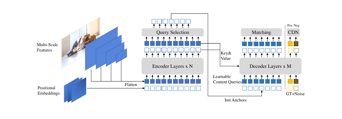
DINO attacks both. The technical contributions target three separate places where the DAB-DETR + DN-DETR baseline still wastes capacity: the one-to-one matching (anchors near a GT box are ambiguous and produce duplicates), the query initialization (encoder-selected content queries are unrefined and can mislead the decoder), and the box refinement (Deformable DETR’s gradient detachment means an early layer’s initial box never receives a corrective signal from later layers).

Preliminaries: what DINO inherits

• From DAB-DETR (DAB-DETR): decoder positional queries are explicit 4D dynamic anchor boxes $(x,y,w,h)$, refined layer by layer in the decoder, rather than opaque learned embeddings. This makes “what a query is” concrete, and makes anchor-space reasoning (noise scales, IoU, refinement) possible at all.
• From DN-DETR (DN-DETR): an auxiliary denoising branch. Noised GT labels and boxes are fed to the decoder alongside the ordinary queries, and the model is trained to reconstruct the originals. The added noise is bounded by $|\Delta x|<\frac{\lambda w}{2}$, $|\Delta y|<\frac{\lambda h}{2}$, $|\Delta w|<\lambda w$, $|\Delta h|<\lambda h$. A noised GT box is just an anchor with a GT box nearby, so this trains the decoder’s “refine a nearby anchor” skill directly, bypassing the instability of bipartite matching in early training.
• From Deformable DETR: multi-scale deformable attention for efficiency, query selection (the paper deliberately renames Deformable DETR’s “two-stage” to avoid confusion with classical two-stage detectors), and iterative box refinement with gradient detachment — which DINO renames look forward once.

Model overview

Standard DETR-like skeleton: backbone (ResNet-50 or SwinL) → multi-scale features → 6-layer deformable Transformer encoder → 6-layer deformable Transformer decoder → prediction heads. The decoder’s positional queries are dynamic anchor boxes; its content queries are learnable parameters. Two query streams run through the decoder in parallel: the ordinary matching queries and the CDN (contrastive denoising) queries.

Contrastive denoising training

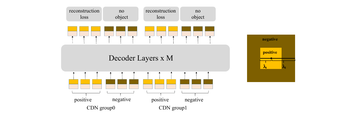
DN-DETR teaches the model to reconstruct a GT box from a nearby anchor. What it never teaches is to say “no object” for an anchor that has no object nearby — every DN query has a GT target by construction. The consequence is duplicate predictions: several anchors sit close to one object, the model cannot decide which to use, and self-attention’s duplicate-suppression is only partially effective.

CDN fixes this by generating, per GT box, two noised queries with two noise scales ${\lambda }_1<{\lambda }_2$:

• Positive queries — noise scale smaller than ${\lambda }_1$; inside the inner square in the concentric-square picture. Target: reconstruct the corresponding GT box.
• Negative queries — noise scale between ${\lambda }_1$ and ${\lambda }_2$; in the ring between the inner and outer square. Target: “no object”.

${\lambda }_2$ is kept small deliberately — hard negatives, close to the GT box, are the informative ones. An image with $n$ GT boxes yields a CDN group of $2n$ queries, and (as in DN-DETR) multiple CDN groups are used per image. Losses: ${\ell }_1$ + GIoU for box reconstruction and focal loss for classification, with the negatives’ background classification also using focal loss.

The mechanism is anchor selection rather than anchor regression: the model learns to reject useless anchors instead of merely pulling every anchor toward the nearest GT. That removes duplicates (Fig. 8 in the paper shows a person with 3 duplicate boxes under DN queries and one box under CDN queries) and stops unwanted far-away anchors from winning the matching.

Measuring it: Average-To-Nearest anchor distance

To show CDN actually improves the anchors rather than just the loss curve, the paper defines ATD(k). For each GT box $b_i=(x_i,y_i,w_i,h_i)$ in the validation set, let $a_i=(x_i^{\prime },y_i^{\prime },w_i^{\prime },h_i^{\prime })$ be the initial decoder anchor whose final refined box was matched to $b_i$. Then

$ATD(k)=\frac{1}{k}\sum \left\{topK(\{\Vert b_0-a_0{\Vert }_1,\Vert b_1-a_1{\Vert }_1,\dots ,\Vert b_{N-1}-a_{N-1}{\Vert }_1\},k)\right\}$

i.e. the mean ${\ell }_1$ anchor–GT distance over the $k$ worst pairs. The top-$k$ restriction is the point: confusion happens precisely when a GT box gets matched to a far anchor, so the tail is what matters. DN alone already gives a good average anchor; CDN specifically improves the tail and does so most for small objects, worth $+1.3$ AP${}_S$ over DN queries at 12 epochs with ResNet-50 and multi-scale features.

Mixed query selection

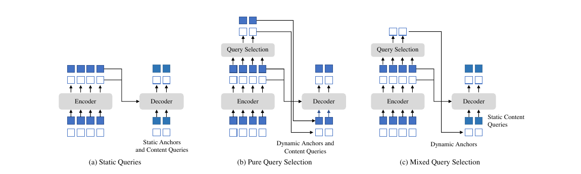
Three ways to initialize decoder queries, given that a query has a positional part (anchor) and a content part:

• (a) Static queries — DETR, DN-DETR, DAB-DETR. Both parts are learned parameters, identical for every image. No encoder information enters the initialization.
• (b) Pure query selection — Deformable DETR’s “two-stage”, and Efficient DETR. Top-$K$ encoder features (by objectness score) initialize both the anchors and the content queries, and are additionally fed to an auxiliary detection head to produce the initial reference boxes.
• (c) Mixed query selection — DINO. Only the positional queries are initialized from the top-$K$ selected features’ position information; content queries stay learnable and static.

The argument against (b): the selected encoder features are preliminary, unrefined content. A selected feature may straddle multiple objects or cover only part of one, so using it as a content query actively misleads the decoder. Its position, on the other hand, is a reliable prior. Keeping the content queries learnable lets the first decoder layer focus on the spatial prior and pool its own, more comprehensive content features from the encoder via cross-attention.

Look forward twice

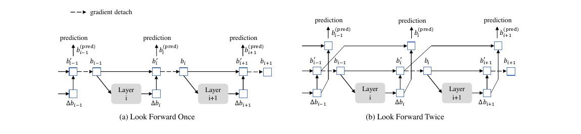
Deformable DETR’s iterative box refinement blocks gradient back-propagation through the box passed between layers, to stabilize training — DINO calls this look forward once, since layer $i$‘s parameters are updated only by the auxiliary loss on its own box $b_i$.

The precision of a predicted box $b_i^{(\text{pred})}$ depends on two things: the quality of the initial box $b_{i-1}$ coming in, and the quality of the predicted offset $\Delta b_i$. Look forward once optimizes only the second, because the gradient path through ${\sigma }^{-1}(b_{i-1})$ is severed. DINO’s look forward twice supervises layer $i$‘s box with the next layer’s output too, so each predicted offset $\Delta b_i$ is used twice — once for $b_i^{\prime }$ and once for $b_{i+1}^{(\text{pred})}$. Given an input box $b_{i-1}$:

$\Delta b_i={\text{Layer}}_i(b_{i-1}),b_i^{\prime }=\text{Update}(b_{i-1},\Delta b_i)$

$b_i=\text{Detach}(b_i^{\prime }),b_i^{(\text{pred})}=\text{Update}(b_{i-1}^{\prime },\Delta b_i)$

where $b_i^{\prime }$ is the undetached version of $b_i$ and $\text{Update}(\cdot ,\cdot )$ is Deformable DETR’s box update — sum in inverse-sigmoid space, then sigmoid, exactly the $\sigma (\Delta +{\sigma }^{-1}(\cdot ))$ construction described in Deformable DETR. So the prediction of layer $i$ is formed from the undetached box of layer $i-1$, which lets the loss on layer $i$‘s prediction reach back and improve layer $(i-1)$‘s parameters as well.

Hyperparameters

Reported in Section 4.1 and Appendix D (Table 8).

Setting	Value
Dataset	COCO 2017 (train2017 / val2017 / test-dev)
Backbones	ResNet-50 (ImageNet-1k) and SwinL (ImageNet-22k)
Encoder / decoder layers	6 / 6
Hidden dim	256; FFN dim 2048; 8 heads; dropout 0.0
Deformable sampling points	4 in the encoder, 4 in the decoder
Decoder queries	900 ($300\times 3$ patterns’ worth of compute, vs DN-DETR’s 300 queries with 3 patterns)
Feature scales	4-scale (backbone stages 2–4 + a down-sampled stage-4 map) or 5-scale (+ stage 1)
CDN	${\lambda }_1=1.0$, ${\lambda }_2=2.0$; 100 CDN pairs = 100 positive + 100 negative queries
DN noise	dn_box_noise_scale 0.4, dn_label_noise_ratio 0.5
Optimizer	AdamW, LR $10^{-4}$, backbone LR $10^{-5}$, weight decay $10^{-4}$
Grad clipping	clip_max_norm 0.1
LR schedule	$\times 0.1$ at epoch 11 / 20 / 30 for the 12 / 24 / 36-epoch settings
Batch size	16, on Nvidia A100 GPUs (8 GPUs, batch 2 per GPU)
Matching cost	class 2.0, bbox 5.0, GIoU 2.0
Loss coefficients	classification 1.0, ${\ell }_1$ 5.0, GIoU 2.0; focal loss $\alpha =0.25$, $\gamma =2$
Aux losses	after every decoder layer, plus intermediate losses after the query selection module
Prediction heads	shared across decoder layers (DN-DETR uses unshared heads) — better AP and ~1M fewer parameters
Positional encoding	pe_temperature 20; batch norm frozen (FrozenBatchNorm2d)
Augmentation	DETR’s random crop + scale: shorter side $\in [480,800]$, longer side $\le 1333$

Objects365 pre-training (Appendix D.2): 26 epochs on 64 A100 GPUs (local batch size 1 per GPU, first 5000 val images held out as validation, the rest added to training), then 18 epochs of fine-tuning on train2017 on 16 A100s at $1.5\times$ image size (shorter side 720–1200, longer side $\le 2000$, worth ~0.5 AP), with gradient checkpointing, mixed precision, and 1000 DN queries.

DINO also drops DAB-DETR’s conditional queries (see Conditional DETR) — they did not suit the model — and replaces DN-DETR’s fixed number of DN groups with dynamic DN groups: a fixed number of DN queries per image, with the number of groups adjusted to the image’s object count, since padding to the batch’s largest object count (COCO images have 1–80 objects) is wasteful.

Results

12-epoch ($1\times$) setting, ResNet-50, COCO val2017 (Table 1)

Model	Epochs	AP	AP${}_S$	AP${}_M$	AP${}_L$	GFLOPs	Params	FPS
Faster R-CNN (5scale)	12	37.9	22.4	41.1	49.1	207	40M	21
DETR-DC5	12	15.5	4.3	15.1	26.7	225	41M	20
Deformable DETR (4scale)	12	41.1	—	—	—	196	40M	24
DAB-DETR-DC5	12	38.0	19.2	40.9	55.4	256	44M	17
Dynamic Head (5scale)	12	43.0	24.7	46.4	53.9	—	—	—
DN-Deformable-DETR (4scale)	12	43.4	24.8	46.8	59.4	265	48M	23
DINO-4scale	12	49.0 ($+5.6$)	32.0 ($+7.2$)	52.3	63.0	279	47M	24
DINO-5scale	12	49.4 ($+6.0$)	32.3 ($+7.5$)	52.5	63.9	860	47M	10

The small-object gain ($+7.2$ / $+7.5$ AP${}_S$) is disproportionately large, consistent with the CDN/ATD analysis. The 4-scale model adds negligible compute and parameters over DN-Deformable-DETR while running slightly faster.

Longer schedules (Table 2)

Model	Epochs	AP	AP${}_S$	AP${}_M$	AP${}_L$
Faster R-CNN	108	42.0	26.6	45.4	53.4
DETR-DC5	500	43.3	22.5	47.3	61.1
Deformable DETR	50	46.2	28.8	49.2	61.7
DAB-Deformable-DETR	50	46.9	30.1	50.4	62.5
DN-Deformable-DETR	50	48.6	31.0	52.0	63.7
DINO-4scale	24	50.4 ($+1.8$)	33.3	53.7	64.8
DINO-5scale	24	51.3 ($+2.7$)	34.5	54.2	65.3
DINO-4scale	36	50.9 ($+2.3$)	34.6	54.1	64.6
DINO-5scale	36	51.2 ($+2.6$)	35.0	54.3	65.3

Because DINO converges fast, the paper uses the $2\times$/$3\times$ (24/36-epoch) settings rather than the usual 50 — the extra epochs buy very little (51.3 at 24 vs 51.2 at 36 for 5-scale).

SOTA comparison (Table 3, SwinL + Objects365)

Method	Params	Backbone pre-train	Detection pre-train	Uses mask	End-to-end	val2017 AP (no TTA)	test-dev AP (no TTA)
SwinL	284M	IN-22K-14M	O365	✓		57.1	57.7
Soft Teacher + SwinL	284M	IN-22K-14M	O365	✓		60.1	61.3
Florence-CoSwin-H	> 637M	FLD-900M	FLD-9M			—	62.4
SwinV2-G	3.0B	IN-22K-ext-70M	O365	✓		61.9	63.1
DINO-SwinL	218M	IN-22K-14M	O365		✓	63.2	63.3

Relative to SwinV2-G: $1/15$ the parameters. Relative to Florence: $1/60$ the backbone pre-training images and $1/5$ the detection pre-training data. None of the previous SOTA models use Transformer decoder-based heads, and none are end-to-end (HTC++/DyHead retain RPN and NMS). The 63.2/63.3 numbers are without test-time augmentation; the TTA experiment (Appendix A, using a one-to-one IoU-based weighted-average ensembling scheme instead of NMS/box voting, since DETR-like models are not prone to duplicates and standard ensembling hurts them) gave no inspiring gain.

Component ablation (Table 4, ResNet-50, 12 epochs)

#	Model	QS	CDN	LFT	AP	AP${}_S$	AP${}_M$	AP${}_L$
1	DN-DETR	no			43.4	24.8	46.8	59.4
2	Optimized DN-DETR	no			44.9	26.9	48.2	60.0
3	Strong baseline (row 2 + pure query selection)	pure			46.5	29.6	49.8	61.0
4	+ mixed query selection	mixed			47.0	31.1	50.1	61.5
5	+ look forward twice	mixed		✓	47.4	29.9	50.8	61.9
6	DINO (+ contrastive DN)	mixed	✓	✓	47.9	31.2	50.9	61.9

Engineering and pipeline optimization account for $+1.5$ AP (43.4 → 44.9), pure query selection for $+1.6$, and the three novel components for $+0.5$, $+0.4$ and $+0.5$ respectively — roughly $+1.4$ AP in total on an already strong baseline.

Other ablations

Encoder/decoder depth (Table 6, 12 epochs, 100 DN queries without negatives): 6/6 → 47.4; 4/6 → 46.2; 3/6 → 45.8; 2/6 → 45.4; 6/4 → 46.0; 6/2 → 44.4; 2/4 → 44.1; 2/2 → 41.2. Cutting decoder layers hurts more than cutting encoder layers, since the boxes are refined through each decoder layer — but DINO degrades far more gracefully than Dynamic DETR (3.0 AP drop going 6→2 decoder layers vs 13.8 AP, 29.1 vs 42.9), which the paper credits to mixed query selection giving well-initialized decoder queries that are not deeply coupled to refinement depth.

Number of denoising queries (Table 7): 100 CDN (= 200 queries: 100 positive + 100 negative) → 47.9; 1000 DN → 47.6; 200 DN → 47.4; 100 DN → 47.4; 50 DN → 46.7; 10 DN → 46.0; no DN → 45.1. Denoising is worth ~2.8 AP, saturates around 100 queries, and past that more DN queries do nothing or slightly hurt.

Training efficiency (Table 5, 8× A100, ResNet-50): ~55 min/epoch, 16 GB GPU memory, 12 epochs to 47.9 AP — versus Deformable DETR at ~55 min/epoch × 50 epochs to 45.4, DETR at ~16 min/epoch × 300 epochs (26 GB) to 41.2, and Faster R-CNN at ~60 min/epoch × 108 epochs to 42.0.

Limitations

• The three contributions are individually small ($+0.5$, $+0.4$, $+0.5$ AP in the ablation); most of the headline gap over DN-Deformable-DETR comes from the engineering-optimized baseline and query selection. The paper is as much a strong-recipe paper as a new-mechanism paper.
• The 5-scale model costs 860 GFLOPs and runs at 10 FPS (vs 279 GFLOPs / 24 FPS for 4-scale) for $+0.4$ AP at 12 epochs — the high-resolution level is expensive for what it buys.
• CDN adds hyperparameters (${\lambda }_1$, ${\lambda }_2$, group count, DN query budget) with no principled way to pick them; the paper only reports that ${\lambda }_2$ should be small and 100 CDN pairs is a good point on the saturation curve.
• The SOTA result depends on Objects365 pre-training on 64 A100s for 26 epochs — the leaderboard number is not reproducible on a modest budget, and the ResNet-50 results are the honest comparison point.
• Test-time augmentation, which reliably helps classical detectors, gives no meaningful gain here; DETR-like models resist the usual ensembling machinery because their set-based loss already suppresses duplicates.
• Inference still inherits Deformable DETR’s custom CUDA kernel for multi-scale deformable attention and its unordered memory access.

See also

• DETR — the set-prediction formulation DINO is built on
• Deformable DETR — supplies the multi-scale deformable attention, query selection, and the “look forward once” refinement DINO improves
• DAB-DETR — dynamic anchor-box queries, the formulation that makes CDN’s noise scales meaningful
• DN-DETR — denoising training, which CDN extends with negative samples
• Conditional DETR — the conditional spatial query, which DINO evaluated and dropped
• RT-DETR — the real-time descendant of this line
• Implementing Research Papers