LW-DETR

LW-DETR (Light-Weight DEtection TRansformer) is a real-time detection transformer.

• Paper: Chen, Su, Zhang, Wang, Chen, Shen, Han, Chen, Xu, Li, Zhang, Yao, Ding, Zhang and Wang (Baidu Inc. and collaborators), LW-DETR: A Transformer Replacement to YOLO for Real-Time Detection, June 2024, arXiv:2406.03459.
• Architecture: where RT-DETR keeps a convolutional backbone and rebuilds the DETR encoder, LW-DETR goes the other way: the encoder is a plain ViT, and the whole detector is a three-part stack, ViT encoder → convolutional projector → shallow DETR decoder.
• Contribution: no architectural invention at all; a careful assembly of existing techniques.
• Training-effective techniques: Objects365 pre-training, IA-BCE loss, Group DETR supervision, deformable cross-attention.
• Inference-efficient techniques: interleaved window/global attention, window-major feature map organization, a 3-layer decoder.
• Headline result: five models spanning 42.6 mAP at 500 FPS (tiny) to 58.3 mAP at 52 FPS (xlarge) on COCO val2017, T4 + TensorRT FP16, dominating YOLO-NAS, YOLOv8, RTMDet, YOLOv10 and RT-DETR at every scale.

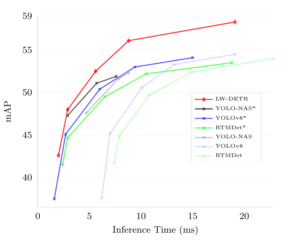
The starred curves are the competitors with their NMS score threshold tuned by the authors rather than left at the official default — i.e. the baselines are strengthened, not weakened, before the comparison. LW-DETR is above all of them across the whole latency range.

Core idea: a plain ViT is a viable real-time detection backbone

The premise the paper tests is that the DETR line’s real-time problem was never the transformer as such, but the specific way DETRs were built. The received wisdom by 2024 was that real-time detection needs a convolutional backbone (every YOLO, and RT-DETR too), because global self-attention is quadratic in the number of patches. LW-DETR argues that a plain ViT encoder becomes affordable once you (a) replace most global attention layers with window attention, (b) implement that replacement without the permutation overhead the standard ViTDet implementation incurs, and (c) shorten the decoder from the customary 6 layers to 3.

The second premise, and empirically the larger one, is that detection transformers benefit far more from large-scale pre-training than convolutional detectors do. Objects365 pre-training is worth $+5.5$ mAP on average across the LW-DETR scales — a gain the YOLO-family baselines simply do not get (see Pre-training below).

Architecture

LW-DETR is exactly three components.

ViT encoder

A plain ViT: a patchification layer plus transformer encoder layers, each a multi-head self-attention followed by an FFN. Two modifications:

Multi-level feature map aggregation. Instead of feeding the decoder only the last layer’s output, the encoder aggregates intermediate and final feature maps into one richer encoded map. Because a plain ViT is isotropic — every layer has the same spatial resolution — this is a plain concatenation, not a feature pyramid; there is no resampling involved.

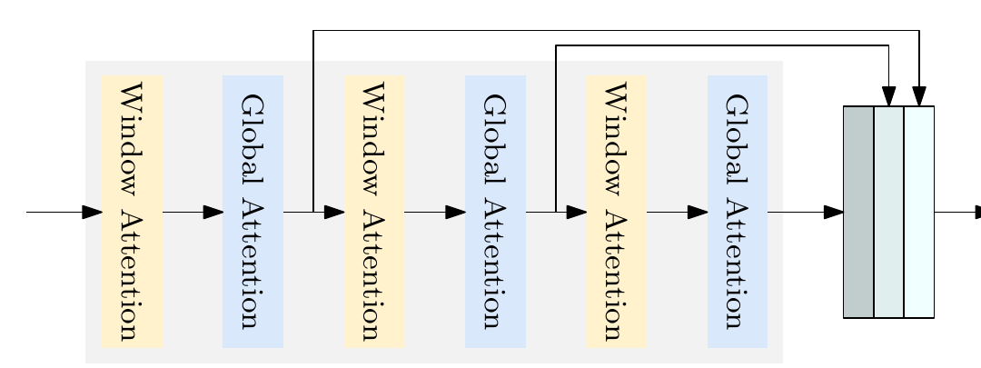
Interleaved window and global attention. Some global self-attention layers are replaced with window self-attention, which partitions the feature map into non-overlapping windows and attends within each. In the 6-layer tiny encoder, layers 0, 2 and 4 are window layers; in the 10-layer small/medium/large/xlarge encoders it is layers 0, 1, 3, 6, 7. The number of windows is fixed at 16 across image resolutions rather than the window size being fixed — which is why the input must be divisible by the window count, and why the paper uses a $10\times 10$ window size at $640\times 640$.

Projector

A C2f block — the cross-stage-partial DenseNet extension used in YOLOv8 — connecting encoder to decoder. Its job is channel reduction and a little convolutional mixing on the aggregated encoded feature maps.

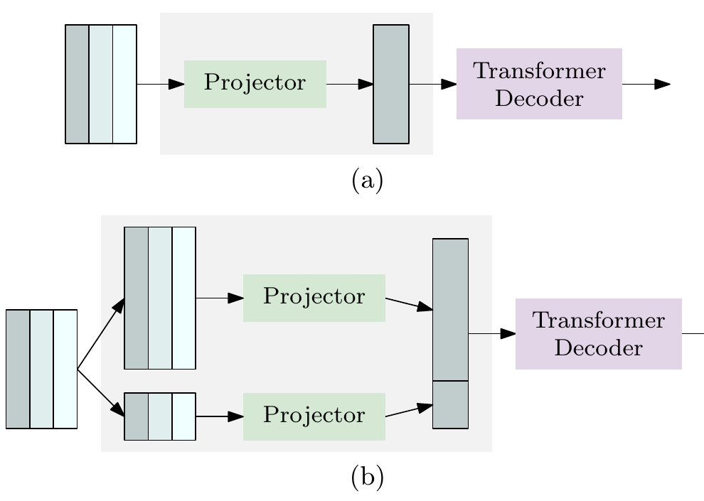
For tiny/small/medium the projector is single-scale: one C2f block, one output map at $\frac{1}{16}$ resolution. For large/xlarge it outputs two scales, $\frac{1}{8}$ and $\frac{1}{32}$, via two parallel C2f blocks — one path upsamples the $\frac{1}{16}$ input with a deconvolution, the other downsamples it with a strided convolution — and the decoder becomes the multi-scale deformable decoder of Deformable DETR.

Decoder

A stack of transformer decoder layers, each self-attention → cross-attention → FFN, with deformable cross-attention (Deformable DETR) for efficiency. The critical departure from DETR convention is depth: 3 layers, not 6. On the tiny model this cuts decoder time from 1.4 ms to 0.7 ms, against 1.3 ms for everything else — so it is roughly a 25% end-to-end saving, not a rounding error.

Queries follow DINO’s mixed query selection: each object query is the sum of a content query (a learnable embedding, as in DETR) and a spatial query obtained two-stage — take the top-$K$ features from the projector’s last layer, predict boxes from them, and embed those boxes as spatial queries. Content queries stay static, spatial queries are data-dependent.

Objective function

The classification loss is the IA-BCE loss (IoU-aware binary cross-entropy) from Align-DETR:

${\ell }_{\text{cls}}={\sum }_{i=1}^{N_{pos}}\mathrm{BCE}(s_i,t_i)+{\sum }_{j=1}^{N_{neg}}{s}_j^2\mathrm{BCE}(s_j,0)$

where $s$ is the predicted classification score and the positive target $t$ absorbs the IoU $u$ against the ground truth:

$t=s^{\alpha }{u}^{1-\alpha },\alpha =0.25$

The target score is thus a geometric mean of the model’s own confidence and its localization quality, so a confidently-classified but badly-localized prediction is trained down. The negative term is weighted by $s_j^2$, a focal-style down-weighting of easy negatives. This is the same classification/localization alignment idea as Task-Aligned-Assignment and RT-DETR’s uncertainty-minimal query selection, applied here to the loss target.

The total loss adds the standard DETR box terms:

${\ell }_{\text{cls}}+{\lambda }_{\text{iou}}{\ell }_{\text{iou}}+{\lambda }_{{\ell }_1}{\ell }_1,{\lambda }_{\text{iou}}=2.0,{\lambda }_{{\ell }_1}=5.0$

with ${\ell }_{\text{iou}}$ the GIoU loss and ${\ell }_1$ the L1 box loss.

Box regression reparameterization. Rather than regressing box coordinates directly, each decoder layer predicts a transformation $[{\delta }_x,{\delta }_y,{\delta }_w,{\delta }_h]$ applied to a proposal $[p_{c_x},p_{c_y},p_w,p_h]$:

$b_{c_x}={\delta }_x{p}_w+p_{c_x},b_{c_y}={\delta }_y{p}_h+p_{c_y},b_w=\exp ({\delta }_w)p_w,b_h=\exp ({\delta }_h)p_h$

the standard two-stage-detector parameterization, imported into DETR.

Effective training

Group DETR supervision. LW-DETR uses 13 parallel weight-sharing decoders during training, each with its own group of object queries generated from the projector output, following Group DETR. Only the primary decoder is used at inference, so this is free at test time — the same “extra supervision without inference cost” trick as DN-DETR’s denoising branch, from a different direction.

Two-stage Objects365 pre-training. First the ViT alone is pre-trained on Objects365 with the MIM method CAEv2 (worth $+0.7$ mAP on COCO over the ImageNet weights); then the encoder is retrained and the projector and decoder trained in a supervised way on Objects365, following Group DETR v2. Only then does COCO fine-tuning start.

Efficient inference: window-major feature map organization

This is the paper’s one genuinely novel implementation detail, and the empirical study shows why it matters. Interleaved window/global attention cuts small’s FLOPs from 23.0G to 16.6G — a 28% reduction — but in the ViTDet implementation the latency actually rises by 0.2 ms. The reason is that ViTDet stores feature maps row-major, so every window-attention layer must permute memory into window order and back, and the permutation costs more than the saved attention.

LW-DETR instead stores the feature map window-major from the start. For a $4\times 4$ map

$\left[\begin{array}{cccc}{f}_{11}& f_{12}& f_{13}& f_{14}\\ f_{21}& f_{22}& f_{23}& f_{24}\\ f_{31}& f_{32}& f_{33}& f_{34}\\ f_{41}& f_{42}& f_{43}& f_{44}\end{array}\right]$

with window size $2\times 2$, the window-major order is

$f_{11},f_{12},f_{21},f_{22};f_{13},f_{14},f_{23},f_{24};f_{31},f_{32},f_{41},f_{42};f_{33},f_{34},f_{43},f_{44}$

rather than the row-major

$f_{11},f_{12},f_{13},f_{14};f_{21},f_{22},f_{23},f_{24};\dots$

Window attention over the window-major layout is a contiguous read, and global attention is order-agnostic, so both work without any permutation. Latency drops from 3.7 ms to 2.9 ms — a 0.8 ms saving that is larger than the entire decoder-shortening gain.

Instantiations

Five detectors (Table 1):

	Encoder layers	Encoder dim	Global attn.	Window attn.	Projector blocks	Projector dim	Scales	Decoder layers	Queries
tiny	6	192	3	3	1	256	$\frac{1}{16}$	3	100
small	10	192	4	6	1	256	$\frac{1}{16}$	3	300
medium	10	384	4	6	1	256	$\frac{1}{16}$	3	300
large	10	384	4	6	1	384	$\frac{1}{8},\frac{1}{32}$	3	300
xlarge	10	768	4	6	1	384	$\frac{1}{8},\frac{1}{32}$	3	300

Note that the decoder is 3 layers at every scale — the family scales through encoder width and projector scales only.

Hyperparameters

Objects365 pre-training (Table 9):

Setting	Value
Optimizer	AdamW
Base LR	$4.0\times 10^{-4}$
Encoder LR	$6.0\times 10^{-4}$
Weight decay	$1\times 10^{-4}$
Batch size	128
Epochs	30
Training image resolutions	$\{448,512,576,640,704,768,832,896\}$
Encoder layer-wise LR decay	0.8 (T/S), 0.7 (M/L), 0.75 (X)
Encoder layers	6 (T), 10 (S/M/L/X)
Drop path	0 (T/S/M), 0.05 (L/X)
Window numbers	16
Window attention indexes	$[0,2,4]$ (T), $[0,1,3,6,7]$ (S/M/L/X)
Output feature indexes	$[0,2,4]$ (T), $[2,4,5,9]$ (S/M/L/X)
Feature scales	$\frac{1}{16}$ (T/S/M), $\{\frac{1}{8},\frac{1}{32}\}$ (L/X)
Object queries	100 (T), 300 (S/M/L/X)
Decoder layers	3
Hidden dimensions	256 (T/S/M), 384 (L/X)
Decoder self-attention heads	8 (T/S/M), 12 (L/X)
Decoder cross-attention heads	16 (T/S/M), 24 (L/X)
Decoder sampling points	2 (T/S/M), 4 (L/X)
Group DETR groups	13
EMA decay	0.9997

There is no LR drop schedule — the initial learning rate is held for the whole pre-training run.

COCO fine-tuning (Table 10) — the modifications on top of the above:

Setting	Value
Base LR	$1.0\times 10^{-4}$
Encoder LR	$1.5\times 10^{-4}$
Weight decay	$1\times 10^{-4}$ (T/S/M/L), $1\times 10^{-3}$ (X)
Batch size	32 (T/S/M), 16 (L/X)
Epochs	50 (T/S/M), 25 (L/X) — 180K iterations total
Drop path	0 (T/S/M), 0.1 (L/X)
Component-wise LR decay	0.7 (T/S/M), 0.5 (L/X)
Input resolution	$640\times 640$

Component-wise LR decay gives different scale factors to the prediction heads, the DETR decoder layers, the projector and the ViT encoder respectively: with a factor of 0.7 the scales are $0.7^0$, $0.7^1$, $0.7^2$, $0.7^3$ — i.e. the encoder learns 3.4× slower than the heads.

Latency throughout is measured end-to-end, FP16, batch size 1, on a T4 with TensorRT-8.6.1 / CUDA-11.6 / cuDNN-8.7.0, using the efficientNMSPlugin for the NMS-based baselines.

Results

Empirical study: where the mAP comes from

Table 2 builds small from an all-global-attention initial detector, one technique at a time (45K iterations = 12 epochs, except the final row at 180K):

Setting	Params (M)	FLOPs (G)	Latency (ms)	mAP
Initial detector	10.8	22.8	3.6	35.3
+ multi-level feature aggregation	11.0	23.0	3.7	36.0
+ interleaved window/global attention (ViTDet impl.)	11.0	16.6	3.9	34.7
+ window-major feature map organization	11.0	16.6	2.9	34.7
+ IoU-aware classification loss	11.0	16.6	2.9	35.4
+ more supervision (Group DETR)	14.6	16.6	2.9	38.4
+ bounding box reparameterization	14.6	16.6	2.9	38.6
+ pre-training on Objects365	14.6	16.6	2.9	47.3
LW-DETR-small (180K iterations)	14.6	16.6	2.9	48.0

Two things stand out. First, the latency story is entirely the window-major reorganization: interleaved attention alone loses 0.2 ms despite a 28% FLOP cut; the reorganization recovers that and 0.6 ms more. Second, the accuracy story is overwhelmingly pre-training: $+8.7$ mAP from Objects365 against $+3.0$ for Group DETR, $+0.7$ each for feature aggregation and IA-BCE, and $+0.2$ for box reparameterization. Architecture contributes single-digit tenths; data contributes 8.7 points.

Against real-time detectors

COCO val2017, T4 + TensorRT FP16, batch 1, total latency including NMS where applicable (Table 3, selected rows; all LW-DETR rows use Objects365 pre-training):

Method	Params (M)	FLOPs (G)	Model latency (ms)	Total latency (ms)	mAP
RTMDet-t	4.9	8.1	2.1	7.4	41.7
YOLOv8n	3.2	4.4	1.5	6.2	37.6
LW-DETR-tiny	12.1	11.2	2.0	2.0	42.6
RTMDet-s	8.9	14.8	2.8	7.9	44.9
YOLOv8s	11.2	14.4	2.6	7.0	45.2
YOLO-NAS-s	19.0	17.6	2.8	4.7	47.6
LW-DETR-small	14.6	16.6	2.9	2.9	48.0
YOLO-NAS-m	51.1	48.0	5.5	7.8	51.6
LW-DETR-medium	28.2	42.8	5.6	5.6	52.5
YOLOv8l	43.7	82.7	9.3	13.2	53.3
YOLO-NAS-l	66.9	65.5	7.5	8.8	52.3
LW-DETR-large	46.8	71.6	8.8	8.8	56.1
YOLOv8x	68.2	129.3	14.8	19.1	54.5
LW-DETR-xlarge	118.0	174.2	19.1	19.1	58.3

Being NMS-free, LW-DETR’s total latency equals its model latency — the column that costs YOLOv8n 4.7 ms and RTMDet-t 5.3 ms. Against YOLO-NAS, the strongest baseline (itself the product of a neural architecture search), LW-DETR gains 0.4 mAP at 1.6× the speed at small, 0.9 mAP at ~1.4× at medium, and 3.8 mAP at equal speed at large — the margin widens with scale.

Against concurrent work

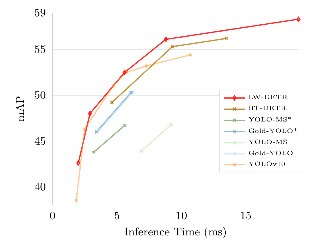
From Table 4:

Method	Params (M)	FLOPs (G)	Total latency (ms)	mAP
YOLOv10-S	7.2	21.6	2.49	46.3
YOLOv10-L	24.4	120.3	7.28	53.2
YOLOv10-X	29.5	160.4	10.70	54.4
RT-DETR-R18 (O365)	20	30.0	4.6	49.2
RT-DETR-R50 (O365)	42	69.4	9.3	55.3
RT-DETR-R101 (O365)	76	131.0	13.5	56.2
LW-DETR-small	14.6	16.6	2.9	48.0
LW-DETR-large	46.8	71.6	8.8	56.1
LW-DETR-xlarge	118.0	174.2	19.1	58.3

LW-DETR-large beats RT-DETR-R50 by 0.8 mAP while being faster (8.8 ms vs 9.3 ms), and beats YOLOv10-X by 1.7 mAP at lower latency (8.8 ms vs 10.70 ms). Note that YOLOv10’s numbers are without Objects365 pre-training, which is a real asymmetry — but see below for why it may not be one that closes.

Pre-training is the single largest term

Table 5, mAP with and without Objects365 pre-training:

Model	Params (M)	FLOPs (G)	Latency (ms)	w/o pre-training	w/ pre-training	Δ
tiny	12.1	11.2	2.0	36.5	42.6	+6.1
small	14.6	16.6	2.9	43.6	48.0	+4.4
medium	28.2	42.8	5.6	47.2	52.5	+5.3
large	46.8	71.6	8.8	49.5	56.1	+6.6
xlarge	118.0	174.2	19.1	53.0	58.3	+5.3
R18 (conv. encoder)	21.2	21.4	2.5	40.9	44.4	+3.5
R50 (conv. encoder)	54.6	67.7	8.7	49.7	54.4	+4.7

Average $+5.5$ mAP. The comparison that makes this interesting is Table 6, the same experiment on the non-end-to-end detectors as a function of schedule length:

Model	Pre-trained	20 ep	60 ep	100 ep	200 ep	300 ep	500 ep
YOLOv8n		26.2	30.1	32.3	34.0	35.0	37.4
YOLOv8n	✓	31.5	32.8	33.2	34.3	35.2	37.6
RTMDet-t		30.4	34.2	35.2	36.8	41.0	–
RTMDet-t	✓	33.4	36.5	36.7	37.5	41.7	–

Objects365 pre-training gives YOLOv8n $+5.3$ mAP at 20 epochs but only $+0.2$ at 500. Because the YOLO line trains for 300–500 epochs as standard, its published numbers sit exactly where pre-training has stopped helping — the gain is absorbed by the long schedule. LW-DETR, at 50 epochs, is still in the regime where pre-training pays. The paper is explicit that this is a hypothesis with preliminary support, not a settled explanation.

Generalization beyond COCO

Cross-domain, UVO (class-agnostic, 57% of instances outside the 80 COCO classes; models trained on COCO, evaluated directly):

Method	mAP	AP${}_{50}$	AR@100	AR${}_s$	AR${}_m$	AR${}_l$
RTMDet-s	29.7	43.3	55.7	26.5	49.4	71.5
YOLOv8-s	29.1	42.4	54.3	27.4	48.6	68.8
YOLO-NAS-s	31.0	44.5	55.1	25.8	48.1	71.6
LW-DETR-small	32.3	45.1	59.8	29.4	52.4	77.1

$+1.3$ mAP and $+4.1$ AR over the best competitor, with the recall gain present at every object scale — evidence that the advantage is not COCO-specific tuning.

Multi-domain fine-tuning, RF100 (100 small datasets, 7 imagery domains, AP${}_{50}$):

Method	Average	aerial	videogames	microscopic	underwater	documents	electromagnetic	real world
RTMDet-s	79.2	70.1	88.0	68.1	68.0	81.0	77.4	83.3
YOLOv8-s	80.1	70.7	87.9	74.7	70.2	79.8	79.0	82.9
YOLO-NAS-s	81.5	–	–	–	–	–	–	–
LW-DETR-small	82.5	71.8	88.9	74.5	69.6	86.7	84.6	85.3
LW-DETR-medium	83.5	72.9	90.8	75.4	70.5	86.1	86.2	86.4

The margin is concentrated in documents ($+5.7$ AP) and electromagnetic ($+5.6$ AP) — the two domains least like COCO.

Limitations

• The gains are not architectural. By the paper’s own ablation, $8.7$ of the $\sim 12$ mAP the recipe adds to the initial detector come from Objects365 pre-training. Read strictly, LW-DETR demonstrates that a plain-ViT DETR can be made fast, and that pre-training helps DETRs disproportionately — not that this particular stack is better designed than RT-DETR’s.
• The comparison is not schedule-matched. LW-DETR trains 50 epochs (25 for L/X) plus 30 epochs of Objects365; the YOLO baselines train 300–500 epochs on COCO. Table 6 is the paper’s own evidence that this asymmetry is exactly where the advantage lives, which makes the headline comparison harder to read than it looks.
• xlarge scales badly. 118M parameters and 174.2 GFLOPs for 58.3 mAP is 2.5× the parameters of large for $+2.2$ mAP, at 2.2× the latency. The family’s good operating points are small through large.
• Detection only. The paper explicitly scopes itself to real-time detection; open-world detection, multi-person pose estimation and multi-view 3D detection are named as untried future work.
• No multi-scale below large. Three of the five models run a single $\frac{1}{16}$ feature map, and the paper reports no AP${}_S$ breakdown on COCO at all, so the small-object behaviour — historically every DETR’s weak spot, and RT-DETR’s acknowledged one — is not characterized.
• The authors note the recipe is deliberately minimal and that token sparsification, distillation, efficient multi-scale fusion and NAS (as in YOLO-NAS) are all untried on top of it.

See also

• RT-DETR — the concurrent real-time DETR LW-DETR is measured against; the opposite design choice (CNN backbone, redesigned encoder) for the same goal
• DETR Family Comparison — where LW-DETR sits relative to the rest of the line
• DETR — the set-prediction formulation and NMS-free matching that make the end-to-end latency argument possible
• Deformable DETR — supplies the deformable cross-attention in LW-DETR’s decoder and the multi-scale decoder used by large/xlarge
• DINO — source of the mixed query selection scheme
• DN-DETR — the other “extra supervision, zero inference cost” mechanism; Group DETR plays the same role here
• YOLOv8 — the C2f block LW-DETR uses as its projector, and a baseline throughout
• YOLOv10 — the NMS-free YOLO LW-DETR compares against in Table 4
• Task-Aligned-Assignment — the same IoU/classification alignment idea that IA-BCE applies to the loss target
• Implementing Research Papers