EMA

Exponential Moving Average of Weights (EMA)

EMA keeps a second copy of the model whose weights are an exponentially weighted running average of the training weights, and uses that copy — not the raw one — for evaluation and deployment.

• Nature: a training-recipe trick, not a paper; appears in nearly every serious detection, segmentation and classification recipe.
• Lineage: descends from Polyak–Ruppert iterate averaging (Polyak & Juditsky, Acceleration of stochastic approximation by averaging, SIAM J. Control Optim. 1992) and is closely related to Stochastic Weight Averaging (Izmailov et al., arXiv 1803.05407).
• Cost: one extra copy of the weights and one multiply-add per parameter per step; adds nothing at inference.
• Benefit: typically buys a consistent accuracy gain for free.
• Used by: the same update rule, used to build a target rather than a final model, is the momentum teacher in self-distillation and self-supervised learning (see Teacher uses).

Core idea

Let ${\theta }_t$ be the training weights after step $t$ and ${\bar{\theta }}_t$ the EMA weights. After every optimizer step:

${\bar{\theta }}_t=\beta {\bar{\theta }}_{t-1}+(1-\beta ){\theta }_t$

with decay $\beta \in (0,1)$ close to 1 (typically $0.99$–$0.99999$). Unrolling gives an explicit weighted average over past iterates:

${\bar{\theta }}_t=(1-\beta ){\sum }_{k=0}^{t-1}{\beta }^k{\theta }_{t-k}+{\beta }^t{\bar{\theta }}_0$

The snapshot taken $k$ steps ago gets weight $(1-\beta ){\beta }^k$, so the weights sum to $1-{\beta }^t$ and the initialisation ${\bar{\theta }}_0$ takes up the rest. The mean age of the averaged iterates is $\beta /(1-\beta )$, so the effective window is roughly $1/(1-\beta )$ steps: $\beta =0.999$ averages over about the last 1 000 steps, $\beta =0.9999$ over about 10 000.

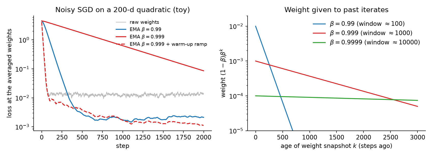
Fig. 1 (toy simulation generated for this page, not a paper result): left — SGD with gradient noise ($\text{lr}=0.05$, $\sigma =1$) plateaus at a noise floor; EMA at $\beta =0.99$ sits roughly $5\times$ lower on that plateau, while plain $\beta =0.999$ is still dominated by the initial weights after 2 000 steps and the warm-up ramp described under Practical details fixes that. Right — the geometric weighting for different decays; the initial weights’ share is ${\beta }^t$.

Why it helps

• Noise reduction. Near a minimum, SGD iterates bounce around it with a variance proportional to the learning rate and gradient noise. Averaging over a window much longer than the iterates’ correlation time cancels most of that noise, so $\bar{\theta }$ sits closer to the centre of the basin than any single ${\theta }_t$ does (left panel of Fig. 1).
• Flatter solutions. The average of several points in a basin tends to lie in a flatter, better-generalising region than the individual points, which is the motivation given for SWA and why the gain shows up on held-out data rather than just training loss.
• Smoother optimisation path. Evaluating the EMA model removes the step-to-step jitter of validation metrics, which also makes checkpoint selection less noisy.

The price is lag: $\bar{\theta }$ trails the current weights by about one window. A decay that is too high for the training length gives an EMA model that is still mostly early-training weights.

Practical details

Warm-up (ramped decay). With ${\bar{\theta }}_0$ set to the random initialisation, a high fixed $\beta$ keeps that initialisation in the average for a long time (the red solid line in Fig. 1). Two common fixes:

• TensorFlow’s ExponentialMovingAverage with num_updates: ${\beta }_t=\min \left(\beta ,\frac{1+t}{10+t}\right)$.
• Ultralytics’ ModelEMA (and timm’s newer EMA variant): ${\beta }_t=\beta (1-e^{-t/\tau })$ with $\tau =2000$ updates, so the decay starts near 0 (EMA ≈ model) and ramps up to $\beta$.

An alternative is Adam-style bias correction, ${\hat{\theta }}_t={\bar{\theta }}_t/(1-{\beta }^t)$, applied when reading the EMA weights instead of when updating them.

Choosing $\beta$. Think in terms of the window $1/(1-\beta )$ relative to the total number of steps. A common rule of thumb is a window of about 1–10 % of training, or a few epochs. Because $\beta$ is applied per step, it must be rescaled when batch size or dataset size changes: to keep a fixed half-life of $h$ samples at batch size $b$, use $\beta =0.5^{b/h}$.

BatchNorm and other buffers. Average every floating-point tensor in state_dict(), including BatchNorm running mean/variance, which is what timm and Ultralytics do; copy integer buffers such as num_batches_tracked. BN statistics from an averaged set of weights are only approximately right; if the EMA model evaluates far worse than the raw one, re-estimating BN statistics on some training batches is the standard check. Models with frozen BN (as in RT-DETR) don’t have this problem.

Evaluation and checkpoints. Always evaluate — and ship — the EMA model; keep the raw weights only to resume training. Save both in the checkpoint, together with the update counter if a warm-up ramp is used.

Cost and distributed training. One extra model copy in memory, and one fused multiply-add per parameter per step (torch._foreach_* / torch._foreach_lerp_ make it cheap). Under DDP every rank holds the same weights after each step, so every rank can maintain its own identical EMA. Under FSDP/ZeRO the EMA must be sharded the same way as the weights.

Interaction with the LR schedule. The benefit is largest with a constant or slowly decayed learning rate (high iterate noise) — LW-DETR pre-trains with no LR drop at all and uses EMA (0.9997). With cosine or linear decay to ~0 the raw iterates already converge and the EMA gain shrinks.

Minimal implementation

A self-contained PyTorch version with the ramped decay (tested: on a small regression run with BatchNorm it reached MSE 0.012 vs 0.088 for the raw weights under the same 300-step SGD run):

import copy
import math
import torch
from torch import nn
 
 
class ModelEMA:
    """Keeps an exponential moving average of a model's weights."""
 
    def __init__(self, model: nn.Module, decay: float = 0.9999, tau: float = 2000.0):
        # The EMA model is a frozen deep copy; it is never trained by the optimizer.
        self.module = copy.deepcopy(model).eval()
        for p in self.module.parameters():
            p.requires_grad_(False)
        self.decay = decay
        self.tau = tau        # warm-up time constant (in updates)
        self.updates = 0
 
    @torch.no_grad()
    def update(self, model: nn.Module):
        """Call once per optimizer step, after optimizer.step()."""
        self.updates += 1
        # Ramp the decay from ~0 up to `decay`: early on the EMA just tracks the
        # model, instead of being dominated by the random initialisation.
        d = self.decay * (1 - math.exp(-self.updates / self.tau))
 
        ema_state, model_state = self.module.state_dict(), model.state_dict()
        for k, v in ema_state.items():
            if v.dtype.is_floating_point:
                # ema = d * ema + (1 - d) * current   (in place, no autograd)
                v.mul_(d).add_(model_state[k].detach(), alpha=1 - d)
            else:
                # integer buffers (e.g. BatchNorm num_batches_tracked): just copy
                v.copy_(model_state[k])
 
 
# --- usage -----------------------------------------------------------------
model = build_model()
ema = ModelEMA(model, decay=0.9999, tau=2000)
opt = torch.optim.AdamW(model.parameters(), lr=1e-4)
 
for x, y in loader:
    loss = criterion(model(x), y)
    opt.zero_grad(); loss.backward(); opt.step()
    ema.update(model)                 # <- the only extra line in the loop
 
evaluate(ema.module, val_loader)      # evaluate / export the EMA model, not `model`
torch.save({"model": model.state_dict(), "ema": ema.module.state_dict(),
            "updates": ema.updates}, "ckpt.pt")

Teacher uses

The update rule is identical, but the averaged network plays a different role: it is a teacher that provides training targets for the live student, so it is used during training rather than only at the end.

• Mean Teacher (Tarvainen & Valpola, NeurIPS 2017, arXiv 1703.01780) — semi-supervised learning: the student is trained on labelled data plus a consistency loss to the EMA teacher’s predictions on unlabelled, differently-perturbed inputs. The EMA teacher is more accurate than the student, so the consistency target improves as training goes on. The paper uses $\beta =0.99$ during an initial ramp-up and $0.999$ afterwards.
• MoCo (He et al., arXiv 1911.05722) — the key encoder producing contrastive keys is an EMA of the query encoder ($m=0.999$), which keeps the queue of stored keys consistent over time.
• BYOL (Grill et al., arXiv 2006.07733) and self-supervised DINO (Caron et al., arXiv 2104.14294) — a stop-gradient EMA teacher gives the target representation; there are no negatives, and the EMA is what keeps the system from collapsing. Both anneal the teacher momentum from 0.996 towards 1 with a cosine schedule. (This DINO is unrelated to the detector in DINO.)
• SigLIP 2 — the local-to-global consistency loss duplicates the image encoder into a student and an EMA teacher that sees the global view while the student sees local crops; see SigLIP2.
• Semi-supervised detection and segmentation (e.g. Unbiased Teacher, Soft Teacher) — the EMA teacher generates pseudo-labels on unlabelled images for the student.

Diffusion models are the other big user of plain (non-teacher) EMA: DDPM (Ho et al., 2020) evaluates EMA weights with $\beta =0.9999$, and because sample quality is very sensitive to the averaging length, EDM2 (Karras et al., arXiv 2312.02696) introduces post-hoc EMA — storing snapshots during training and reconstructing the EMA for any chosen window afterwards.

Hyperparameters

Reported decay values from articles already in this wiki, plus the defaults of the libraries most people actually use. Values in the first block are transcribed from the papers; the library block is from code and is not a paper-stated hyperparameter.

Model / recipe	EMA decay	Notes
RT-DETR	$0.9999$	Listed in its training config
LW-DETR	$0.9997$	Pre-training without any LR drop
CapPa fine-tuning (Image Captioners Are Scalable Vision Learners Too)	$0.99999$ (L/14 @ 336); none for B/16	Together with Polyak averaging, layer-wise LR decay, RandAugment, Mixup
Mean Teacher	$0.99\to 0.999$	Ramp-up phase, then steady state
MoCo	$0.999$	Key encoder momentum
BYOL / self-supervised DINO	$0.996\to 1$	Cosine-annealed teacher momentum
DDPM	$0.9999$	Applied for sampling
Ultralytics ModelEMA (YOLO recipes, e.g. YOLOv8)	$0.9999$, $\tau =2000$	Library default; ramped decay $\beta (1-e^{-t/\tau })$
timm ModelEmaV2	$0.9999$	Library default; no warm-up in V2

Limitations

• Lag at short schedules. A decay tuned for a 300-epoch COCO run is wrong for a 20-epoch fine-tune; the EMA model will still be mostly early weights. Scale the window to the run length.
• Gain depends on the recipe. With a fully annealed LR the raw model is already close to the averaged solution and EMA gives little; it is most useful with constant/slow-decay LR and noisy small-batch training.
• Not a substitute for a good recipe. EMA smooths noise; it does not fix a bad learning rate, too little data, or bad augmentation.
• Resuming. The EMA state and update counter must be checkpointed, otherwise the warm-up restarts and the average is reset.
• BN mismatch. Averaged weights with averaged BN running stats can be slightly inconsistent — check the EMA model against the raw one before trusting it.
• Memory. One more copy of the weights (and of any float buffers), relevant for large models trained near the memory limit.

See also

• RT-DETR — EMA decay 0.9999 in a real-time detector recipe
• LW-DETR — EMA with a constant-LR pre-training schedule
• SigLIP2 — EMA teacher in the local-to-global self-distillation loss
• Image Captioners Are Scalable Vision Learners Too — EMA (Polyak averaging) in the fine-tuning recipe
• How to train your ViT — the wider ViT training-recipe context
• YOLOv8 — Ultralytics recipe, which ships an EMA model by default
• DINO — the detector, whose recipe sits in the same DETR line as RT-DETR
• Implementing Research Papers — checking an EMA implementation when reproducing reported numbers