Image Captioners Are Scalable Vision Learners Too

Image Captioners Are Scalable Vision Learners Too is a compute- and data-matched study showing that pretraining a vision encoder by plain image captioning is a competitive, and in several respects superior, alternative to CLIP-style contrastive pretraining.

• Paper: Michael Tschannen, Manoj Kumar, Andreas Steiner, Xiaohua Zhai, Neil Houlsby and Lucas Beyer (Google DeepMind), NeurIPS 2023, arXiv:2306.07915.
• Models: a standard ViT encoder + Transformer decoder captioning model (Cap) and a mixed autoregressive/parallel-prediction variant (CapPa).
• Setup: both are trained on the same WebLI-derived data, compute budget, and parameter count as the paper’s own re-trained CLIP baselines (denoted CLIP*).
• Headline result: captioning matches or beats contrastive pretraining on classification, and clearly wins on vision-and-language tasks (captioning, OCR, VQA).
• Scaling: equal or better scaling behavior with model size and data.

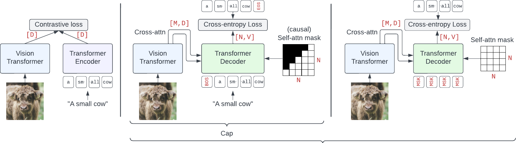
Fig. 1: Contrastive models use two separate encoders matched via a batch-wide contrastive loss. Cap uses an encoder-decoder with causal self-attention and teacher forcing. In parallel decoding (right) the decoder receives an all-[MASK] input and an unmasked self-attention mask, so it must predict every token from the image alone. CapPa alternates between the two regimes during training. $D$: model width, $M$: number of image tokens, $N$: number of text tokens, $V$: vocabulary size.

Motivation: is captioning really an inferior pretraining task?

CLIP established contrastive image-text pretraining as the dominant recipe for building general-purpose vision backbones, and its checkpoints are widely reused as the vision tower in multimodal LLMs (Flamingo, PaLI, PaLM-E, etc.). Generative captioning was explored earlier (VirTex, ICMLM) but was written off as an inferior pretraining signal after CLIP’s original paper showed contrastive zero-shot accuracy scaling much faster with data than captioning did. Subsequent work that does use captioning losses (SimVLM, CoCa, BLIP, GIT, LEMON) mostly does so either at small scale, combined with a contrastive loss, or targeting cross-modal (early-fusion) architectures for VQA/captioning rather than isolating the quality of the resulting vision encoder.

This paper’s contribution is a controlled comparison: same ViT encoder architecture, the same decoder capacity budget (a captioning decoder is half the depth of the encoder so that the Cap model’s total parameter count and per-step accelerator cost roughly match the corresponding CLIP* model, see Table 1 in the paper), the same pretraining data (a deduplicated, English-filtered 1B image/alt-text subset of WebLI), and the same number of training examples seen. Under this regime, next-token captioning turns out to be a much stronger representation learner than the original CLIP paper suggested — the earlier verdict, the authors argue, mostly reflected an unfavorable comparison point rather than an intrinsic weakness of generative pretraining.

Architecture

Both model families reuse a Vision Transformer (ViT) encoder. Cap/CapPa feed the ViT’s output token sequence into a standard Transformer decoder via cross-attention and predict the alt-text tokens (Fig. 1, middle/right); CLIP* instead encodes the text with a separate Transformer encoder and matches image/text embeddings with a batch-wide contrastive loss (Fig. 1, left). Implementation follows recent practice: biases are removed from attention layers, MLP blocks and LayerNorms, and ReLU is replaced by GELU. The decoder has the same width, number of attention heads and MLP dimension as the encoder but only half its depth, and decoder input/output token embeddings are not tied — both ablated in Sec. 4.4 (Table 19) as small but real improvements. This sizing keeps Cap models at a slightly lower total parameter count than the matched CLIP* model while requiring comparable pretraining compute per accelerator-hour (Table 1: B/16 Cap 192M params / 454 TPUv4-hrs per bn. examples vs. B/16 CLIP* 197M / 444 TPUv4-hrs; L/14 Cap 570M / 1570 vs. L/14 CLIP* 640M / 1596).

Key methodology: from Cap to CapPa

Captioner (Cap). Standard next-token-prediction language modeling: the decoder input is the caption shifted right by one token (teacher forcing), a causal self-attention mask enforces autoregressive order, and the training loss is cross-entropy against the target tokens, cross-attending into the frozen sequence of image tokens produced by the ViT encoder.

Parallel prediction (Pa). For a fraction of training examples, the decoder input sequence is replaced entirely by [MASK] tokens and the causal self-attention mask is dropped (full, unmasked self-attention). The decoder must then predict every caption token in a single forward pass, conditioned only on the cross-attended image — no previously-generated tokens are available. This differs from bag-of-words prediction because token position still has to be predicted, not merely presence. Crucially, parallel prediction requires no change to the training objective, decoder architecture, or loss, and — because it only replaces input tokens and the attention mask for a subset of examples — costs no extra compute.

CapPa. The proposed recipe randomly samples, for each training example, whether to use autoregressive (Cap) or parallel (Pa) decoding; the default mixing ratio is 75% parallel-prediction examples, 25% autoregressive, chosen because it gives the most balanced improvement across evaluation datasets (Fig. 6, left) — smaller fractions barely move the needle and larger fractions start hurting some datasets. Alternating parallel/autoregressive per example within a batch is important: doing full-batch parallel prediction for a fraction of batches instead was tried and gave significantly worse results. Only fully-masked parallel sequences were used; masking a random subset of input tokens (leaving partial autoregressive context, as done e.g. by LEMON) did not improve the encoder.

The intuition for why parallel prediction helps the encoder specifically: under pure next-token prediction, the supervisory signal is unevenly distributed across caption positions — early tokens must be predicted almost entirely from the image (strong encoder gradient), while later tokens can increasingly rely on already-generated tokens as context (weaker encoder gradient, since the decoder can partly ignore the image). Under parallel prediction the decoder has no token context at all for any position, so every token in every training example forces it to extract information from the image, giving the encoder a denser, more uniform training signal.

Hyperparameters

Transcribed from Sec. 4.1 and Appendix A.

Pretraining

Data	1B image/alt-text pairs, deduplicated w.r.t. all eval sets, English-filtered subset of WebLI (10B images / 12B multilingual alt-texts)
Batch size	8k for Cap/CapPa; 8k and 16k (CLIP*, to bracket CLIP’s actual training regime)
Examples seen	up to 9B (≈9 epochs over the 1B subset)
Optimizer	AdaFactor variant, cosine LR schedule, 10k warmup steps
Learning rate / decay factor	$10^{-3}$ / $10^{-4}$
Image resolution	$224\times 224$
Text tokenizer	32k-vocabulary SentencePiece model trained on the English portion of C4
Max sequence length	64 tokens
Image tower (CLIP*)	identical architecture/size to the text tower; global average pooling for the image representation
Encoder sizes compared	ViT-S/16, M/16, B/16, L/14

Parallel-prediction mixing (CapPa default)

Fraction of examples with parallel prediction	0.75
Masking	all decoder input tokens replaced with [MASK] (full masking; partial masking did not help)
Self-attention mask under parallel prediction	none (full, unmasked)
Mixing granularity	per example within a batch (per-batch alternation was worse)

Frozen-representation evaluation (10-shot linear/MAP probing, LiT tuning, fine-tuning) hyperparameter sweeps are detailed in Appendix A — full cross-products over epochs $\{1,3,10,30,100\}$, crop strategy, learning rate, weight decay, hidden dimension and loss type were swept per encoder/probe combination; fine-tuning on full ImageNet-1k used AdaFactor with layer-wise LR decay, RandAugment, Mixup and Polyak/EMA averaging, selecting learning rate $10^{-5}$, decay 0.8, Mixup 0.5, no EMA for B/16 and learning rate $10^{-4}$, decay 0.9, EMA 0.99999 for L/14@336.

Results

Frozen representations, single decoder trained from scratch (Table 2 in the paper). CIDEr for captioning, VQAv2 weighted accuracy, exact-match for GQA:

Model	INet 10-shot	COCO CIDEr	Flickr CIDEr	OCR-VQA	VQAv2	GQA
Cap (B/16)	80.2	117.5	78.6	62.2	68.2	55.0
CapPa (B/16)	81.3	117.9	80.5	62.2	68.3	55.7
CLIP* (8k, B/16)	81.1	115.8	74.5	56.0	66.5	54.3
CLIP* (16k, B/16)	81.4	116.3	77.1	56.5	66.7	54.8
CapPa (L/14)	84.4	125.8	89.3	65.6	70.9	58.3
CLIP* (L/14)	84.7	123.2	85.5	61.3	68.5	55.3

CapPa consistently beats Cap, and is competitive with — or (as scale increases) exceeds — CLIP* on classification while clearly winning on captioning, OCR, and VQA even though the decoder in this comparison is a fresh, randomly-initialized one trained from scratch on top of the frozen encoder. The gap widens with model scale: for ViT-L/14, CapPa outperforms CLIP* on most LiT-decoder tasks; for the same encoder, CapPa also clearly beats CLIP* trained at batch size 16k, which is a substantially larger, more favorable contrastive baseline. CapPa’s absolute improvement over CLIP* grows further when the downstream decoder is a frozen, pretrained language model — a T5 decoder with only cross-attention weights retrained gives a much larger CapPa margin than a from-scratch decoder (Fig. 4, left; e.g. up to +10 CIDEr on Flickr, +7.5 exact-match on OCR-VQA), consistent with the intuition that a captioning-pretrained encoder is naturally better matched to being combined with a pretrained text decoder — the setup used by most multimodal LLMs. A frozen GPT-2 decoder combined via a small resampler adapter shows the same direction of improvement but more modestly (Fig. 5).

10-shot linear probing and full fine-tuning. On the pre-logit linear probe (Table 3), CapPa slightly outperforms Cap and is roughly on par with CLIP* trained at batch size 16k; with an MLP or multihead-attention-pooling (MAP) probe instead of a plain linear layer, the small residual gap between captioning-based and contrastive encoders essentially vanishes (Fig. 3) — CLIP*‘s advantage under linear probing is attributed to its training loss inducing linear separability in the average-pooled representation, which a captioning model’s cross-attention-fed decoder does not need. Full fine-tuning on ImageNet-1k gives CLIP* only a small edge (Table 5: CLIP* 84.9/86.0/88.1 vs. CapPa 84.4/85.7/87.7 for B/16, B/16@384, L/14@336).

Zero-shot classification and retrieval via LiT. Fitting a fresh text encoder to the frozen Cap/CapPa image encoder with LiT tuning (Table 4), CapPa is competitive with CLIP* — and for the larger L/14 model, at a given number of LiT examples seen, comes close to or matches it — with typically fewer combined pretraining + LiT-tuning examples than CLIP* uses. This matters because Cap/CapPa’s own decoder is comparatively expensive for zero-shot classification (unlike CLIP’s cached text embeddings, each class name must be scored via a decoder forward pass at inference time), so LiT tuning is the practical route to cheap zero-shot classification/retrieval with a captioning-pretrained encoder.

Word order, attribute and relation sensitivity (ARO, SugarCrepe). On the ARO benchmark (Table 6), Cap and CapPa score near-ceiling on the Flickr/COCO word-order subsets (Order F/C: 99.1–99.2 / 98.7–99.0) and clearly beat CLIP* (45.5 / 37.0) and even NegCLIP, a CLIP variant explicitly fine-tuned for word-order sensitivity — by 8–13 points. On SugarCrepe (Table 7), which fixes known artifacts in ARO, the small B/16 Cap/CapPa models outperform even the largest contrastively-trained G/14 model on every category and essentially solve the “Add” category (plausible-but-wrong additions to a caption), which contrastive bag-of-words-like encoders structurally cannot detect. A “blind” decoder with no image input at all still scores respectably on ARO, showing some of that benchmark’s signal is recoverable from language modeling alone — one motivation for the harder SugarCrepe benchmark.

Fine-grained classification. Transferring the frozen representation with a MAP head to fine-grained datasets (Dogs, Flowers, Birds, Cars, Pets, Food) shows CapPa ahead of CLIP* on most fine-grained tasks and roughly matched on coarse-grained ones (Fig. 4, right; Table 10) — attributed to captioning naturally requiring attention to fine object-level detail to produce an accurate description.

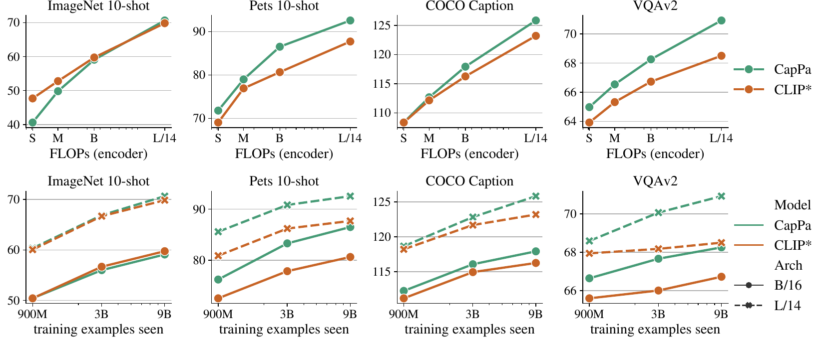
Fig. 2: 10-shot classification (left two columns) and captioning/VQA with a decoder (right two columns), as a function of encoder FLOPs (ViT-S/16 → M/16 → B/16 → L/14, top) and pretraining examples seen (900M → 3B → 9B, bottom). CapPa shows a visibly steeper improvement on captioning and VQA with both axes.

Scaling behavior. Sweeping model size (ViT-S/16 through L/14) and pretraining examples seen (900M to 9B), CapPa and CLIP* scale similarly on classification, but CapPa shows a steeper improvement curve on captioning and VQA metrics along both axes (Fig. 2), suggesting the advantage of captioning-based pretraining should grow further with continued scaling.

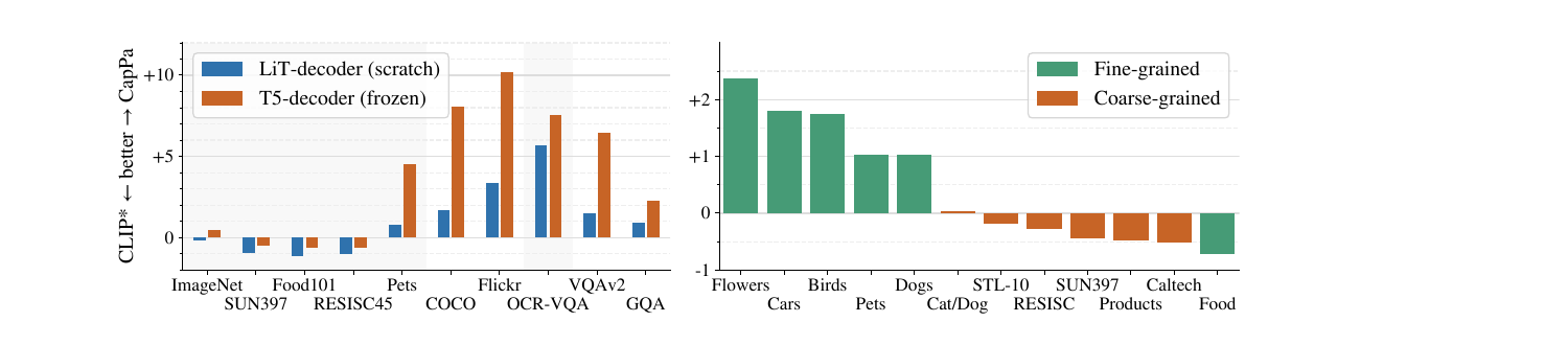
Fig. 4: Left — CapPa’s margin over CLIP* grows substantially when paired with a pretrained, frozen decoder (T5) rather than one trained from scratch (LiT-decoder). Right — CapPa is a better frozen feature extractor on most fine-grained classification datasets.

Ablations

Section 4.4 (all runs at 900M examples seen):

• Parallel-prediction fraction. 0.75 gives the most balanced gain across ImageNet, CIFAR-100, Pets and Cars 10-shot accuracy (Fig. 6, left); very low fractions barely help and full-batch (rather than per-example) parallel-prediction alternation is markedly worse.
• Encoder architecture. Comparing BiT-ResNet50, ViT-B/32 and ViT-B/16 as the encoder, replacing CLIP* with Cap regresses zero-shot/10-shot accuracy least — indeed is roughly neutral — for ViT-B/16, and regresses most for ResNet50 (which produces a spatial grid fed either through cross-attention or, in a “ResNet50 (p)” variant, as a 4-token prefix with no cross-attention at all) (Fig. 6, right). The gap shrinks with ViT and with smaller patch size (i.e., longer token sequences / more FLOPs), independent of parameter count.
• Backward / bidirectional captioning. Randomly reversing the caption 50% of the time (same decoder, same compute) gives no improvement over standard left-to-right Cap (Table 8, left) — differing from prior work’s finding for backward captioning, attributed there to using a separate decoder (differing capacity/FLOPs) rather than a shared one.
• Two decoders instead of decoder mode-switching. A CapPa variant with two independent 3-layer decoders (one per decoding mode, matching the compute of the default 6-layer shared decoder) underperforms the default single-decoder CapPa on most 10-shot tasks (Table 8, left).
• Frozen, language-pretrained decoder. Initializing the decoder from T5-Base and only training cross-attention (optionally also unfreezing the decoder or reinitializing cross-attention) never beats a fully-trained Cap decoder; performance improves monotonically the more the decoder is allowed to deviate from its language-only pretraining (Table 8, right).
• Decoder architectural details. Removing biases from the decoder (as in the encoder) does not hurt and is adopted; using separate input/output token embeddings (rather than tied) helps slightly; six decoder layers is chosen as the depth that best matches the parameter count of the corresponding CLIP* model while remaining strong (Table 19).
• Weight decay / tokenizer variants. Extra weight decay on the decoder or cross-attention layers gave no benefit; retraining the SentencePiece tokenizer on 300M sampled WebLI alt-texts instead of C4 gave no accuracy improvement.
• Pretraining data source. Repeating the comparison on the smaller, differently-curated, CLIP-score-filtered LAION-400M dataset reproduces the main conclusion — CapPa matches CLIP* and outperforms Cap in 10-shot linear evaluation (Fig. 7) — showing the result is not an artifact of WebLI’s particular filtering.

Fig. 6: Left — 10-shot accuracy improvement of CapPa over Cap as a function of the fraction of training examples decoded in parallel; 0.75 balances gains across datasets. Right — improvement (regression) of Cap over CLIP* as a function of encoder architecture; the gap essentially disappears for ViT-B/16.

Limitations

• The Cap/CapPa text decoder itself is of limited standalone use: because it produces a joint autoregressive distribution rather than cached embeddings, zero-shot classification and retrieval require scoring each candidate class/caption with a full decoder forward pass, which is computationally expensive at inference time compared to CLIP’s cached text embeddings — the paper’s own workaround is LiT-tuning a lightweight text encoder on top of the frozen vision backbone.
• On standard zero-shot classification accuracy, Cap/CapPa still generally lag contrastive models, even though the gap narrows with scale — the trade-off documented in the paper is that captioning-based models process fine-grained, word-order-sensitive descriptions much better while contrastive models remain the more efficient zero-shot classifier out of the box.
• Gains from CapPa over CLIP* were not observed under full fine-tuning on ImageNet-1k, where CLIP* keeps a small edge — the benefit of captioning pretraining is clearest for frozen representations, not after further supervised adaptation.
• Parallel prediction is proposed and validated primarily as a representation-learning trick during pretraining; the paper explicitly flags exploring it as an efficient scoring mechanism for downstream zero-shot inference (since a single parallel forward pass scores an entire caption/class jointly) as future work, not something demonstrated here.
• All experiments use a specific compute/parameter matching convention (decoder at half encoder depth, matched training examples); results might shift under different matching conventions or much larger scale than the 9B-example, L/14 regime tested.

See also

• SigLIP — the contrastive pretraining approach (sigmoid loss variant of CLIP) that this paper’s CLIP* baselines are modeled after
• SigLIP2 — a later recipe that folds a captioning-style decoder loss directly into contrastive pretraining, effectively combining both objectives this paper compares in isolation
• How to train your ViT — background on ViT pretraining-recipe choices and data/compute scaling that this paper’s matched-compute methodology builds on
• PaliGemma — a downstream vision-language model where the choice of pretraining objective for the vision encoder (contrastive vs. captioning-influenced) matters for exactly the kind of frozen-decoder combination studied here